5. PRACTICAL REALIZATION OF THE METHOD

s. 72

The detailed design of the electronic circuit that realizes the temperature compensation of transducers according to the new method presented above depends on the type of sensor used. The general circuit design proposed in the remainder of this work, in the form of a multiple bridge, simplifies the design of detailed compensation circuits for all sensors operating in a full-bridge, half-bridge or quarter-bridge configuration.

Since the new method requires that every successive compensating signal $h_{i}(T)$ vanish whenever $h_{i-1}(T) = 0$ , it is proposed that the output signal $H(T)$ of the compensation circuit be generated by means of a chain of bridges. These bridges are connected in such a way that the output voltage on the diagonal of the first bridge is the supply voltage of the second bridge, the output voltage on the diagonal of the second bridge is the supply voltage of the third bridge, and so on. In such a circuit a zero voltage on the diagonal of the first bridge nulls the supply voltages of all the following bridges. We may treat this as a circuit model of the compensating signals $h_{i}(T)$ (see Theorem 1, Section 4.3.1).

In order to make the compensating signals adjustable (the coefficient $w_{i}$ of equation (25)), a potentiometric divider has been introduced into the circuit of each of the bridges mentioned.

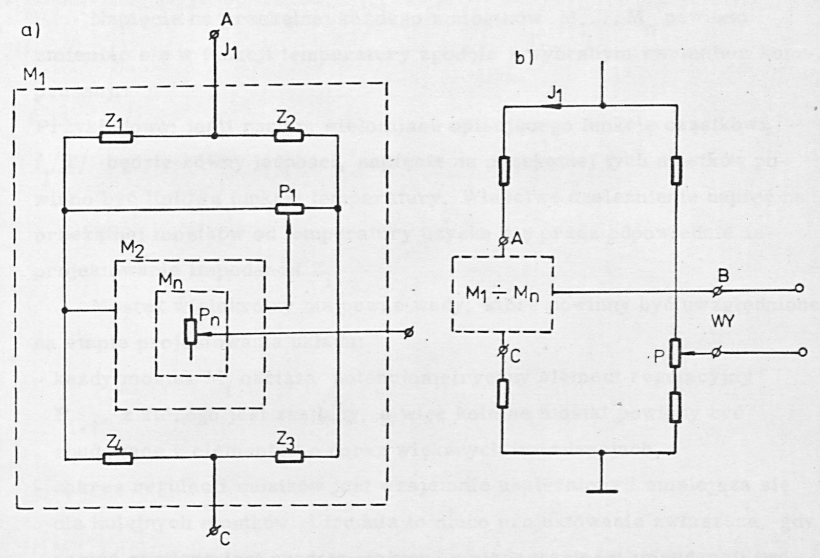
A chain of bridges with the properties described above is called by the author in what follows a "multiple bridge". Fig. 24a shows an example of the construction of such a bridge. The first bridge $M_{1}$ is built of four impedances $Z_{1}$ , $Z_{2}$ , $Z_{3}$ , $Z_{4}$ (frequency- and/or temperature-dependent impedances). A potentiometric divider $P_{1}$ is connected across the bridge diagonal. The potential on one arm of this divider supplies the next bridge $M_{2}$ , built of analogous impedances. A potentiometric divider is connected across the diagonal of bridge $M_{2}$ . The potential of one of its arms supplies bridge $M_{3}$ , and so on. From the last bridge $M_{n}$ the potential of the wiper of the potentiometric divider $P_{n}$ is brought out.¹

Fig. 24. a. General circuit of the multiple bridge b. Method of supplying the bridge

Labels: WY = output (wyjście)

s. 73

The multiple bridge may be connected, for example, into one arm of the measuring bridge (the one containing the sensor) in the manner shown in Fig. 24b; in the other arm there will be a potentiometer P serving to null the bridge signal at the reference temperature. At the successive compensation temperatures the output voltage of the measuring bridge will be nulled by the potentiometric dividers $P_{1} \ldots P_{n}$ .

The voltage on the diagonal of each of the bridges $M_{1} \ldots M_{n}$ should vary as a function of temperature in accordance with the chosen compensation variant: For example: if the degree m of the polynomial describing the component function $f_{j}(T)$ is equal to one, the voltage on the diagonal of these bridges should be a linear function of temperature. The proper dependence of the voltages on the bridge diagonals on temperature is obtained by suitable design of the impedances $Z_{i}$ .

The multiple bridge has certain drawbacks which should be taken into account at the circuit design stage:

each bridge $M_{i}$ loads the potentiometric adjusting element $P_{i-1}$ from which it is supplied, so the successive bridges should be built of components of ever greater impedance,
the adjustment ranges of the bridges are mutually dependent and decrease for the successive bridges. This makes the design somewhat more difficult, especially when the whole is supplied with direct current and the change in the values of the impedances forming the bridge varies as a function of temperature. The use of a computer program for the calculations will then be required,
the input current of the associated circuit of the multiple bridge produces a voltage drop across the equivalent output resistance of the bridge. This resistance changes as the adjusting elements $P_{1}, \ldots, P_{n}$ are adjusted, so the condition for the vanishing of the voltages on the diagonals of the constituent bridges, when the measuring bridge is supplied with a constant voltage, is a function of the wiper position of these elements. To prevent such a dependence it suffices to use a suitably small bridge load current.

s. 74

Because of the drawbacks listed, the bridge multiplicity is limited; nevertheless, obtaining a multiplicity of 1, 2, 3 presents no great difficulty. Below are discussed: the construction and properties of the triple bridge, and also the problem of the interaction between the compensation of the lower and the upper range value.

5.1. Triple bridge

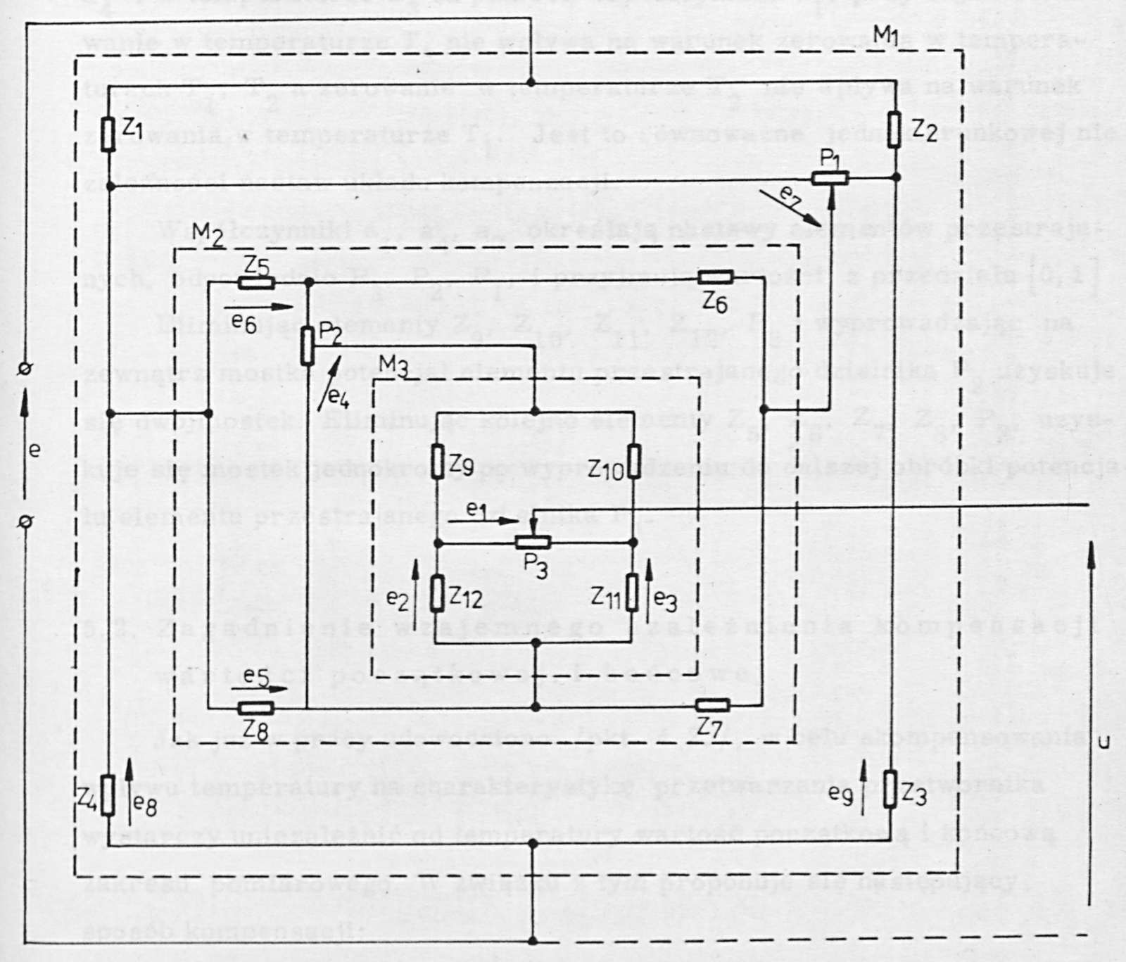
By way of example let us consider a triple bridge (Fig. 25). It is built of three bridges $Z_{1}$ - $Z_{4}$ , $Z_{5}$ - $Z_{8}$ , $Z_{9}$ - $Z_{12}$ . The adjusting elements $P_{1}$ , $P_{2}$ , $P_{3}$ are connected across their respective diagonals. Adopting the notation of Fig. 25, the output voltage of the bridge is determined by the relation:

\frac{u}{e} = a_{8} + a_{5} \cdot a_{7} \cdot (a_{9} - a_{8}) + a_{2} \cdot a_{4} \cdot a_{7} \cdot (a_{6} - a_{5}) \cdot (a_{9} - a_{8}) + a_{1} \cdot a_{4} \cdot a_{7} \cdot (a_{3} - a_{2}) \cdot (a_{6} - a_{5}) \cdot (a_{9} - a_{8}) \qquad (61)

where

e_{1} = a_{1} \cdot (e_{3} - e_{2})

e_{2} = a_{2} \cdot e_{4}

e_{3} = a_{3} \cdot e_{4}

e_{4} = a_{4} \cdot (e_{6} - e_{5})

e_{5} = a_{5} \cdot e_{7}

e_{6} = a_{6} \cdot e_{7}

e_{7} = a_{7} \cdot (e_{9} - e_{8})

e_{8} = a_{8} \cdot e

e_{9} = a_{9} \cdot e

where $a_{1} \ldots a_{9}$ denote the values of the respective division ratios.²

Comparing (61) with (25) we may write

f_{o}(T) = a_{5} \cdot (a_{9} - a_{8}) \cdot e

s. 75

f_{1}(T) = \frac{a_{2}}{a_{5}} \cdot (a_{6} - a_{5}) \cdot e

f_{2}(T) = \frac{1}{a_{2}} \cdot (a_{3} - a_{2}) \cdot e

and

w_{o} = a_{8} \cdot e

w_{1} = a_{7}

w_{2} = a_{4} \cdot a_{7}

w_{3} = a_{1} \cdot a_{4} \cdot a_{7}

Fig. 25. General circuit of the triple bridge

s. 76

Designing the circuit so that: for T = $T_{o}$ :

a_{9} - a_{8} = 0

for T = $T_{1}$ :

a_{6} - a_{5} = 0

for T = $T_{2}$ :

a_{3} - a_{2} = 0

there arises the possibility of nulling the error successively at temperature $T_{1}$ by means of the coefficient $a_{7}$ , at temperature $T_{2}$ by means of the coefficient $a_{4}$ , and at temperature $T_{3}$ by means of the coefficient $a_{1}$ , where nulling at temperature $T_{3}$ does not affect the nulling condition at temperatures $T_{1}$ , $T_{2}$ , and nulling at temperature $T_{2}$ does not affect the nulling condition at temperature $T_{1}$ . This is equivalent to the unidirectional independence of the settings of the compensation circuit. The coefficients $a_{1}$ , $a_{4}$ , $a_{7}$ determine the settings of the adjustable elements $P_{3}$ , $P_{2}$ , $P_{1}$ respectively, and take values from the interval $[0,1]$ . Eliminating the components $Z_{9}$ , $Z_{10}$ , $Z_{11}$ , $Z_{12}$ , $P_{3}$ and bringing the potential of the adjustable element of divider $P_{2}$ out of the bridge, one obtains a double bridge. Eliminating in turn the components $Z_{5}$ , $Z_{6}$ , $Z_{7}$ , $Z_{8}$ , $P_{2}$ , one obtains a single bridge, once the potential of the adjustable element of divider $P_{1}$ has been brought out for further processing.

5.2. The problem of the interaction between the compensation of the lower and the upper range value

As has already been proved in this work (Section 4.2), in order to compensate the effect of temperature on the transfer characteristic of the transducer it suffices to make the lower and the upper range value independent of temperature. In connection with this, the following manner of compensation is proposed:

s. 77

compensation of the temperature drift of one of the values mentioned (the lower or the upper) by bringing the voltage on the diagonal of the measuring bridge to zero. Nulling at the reference temperature would be realized by components placed in one arm of the bridge, whereas nulling at the compensation temperatures would be realized by means of a multiple bridge connected into the other arm of the bridge (Fig. 24b).
compensation of the temperature drift of the other of the values mentioned (the lower or the upper) would be carried out by making the voltage or current supplying the measuring bridge temperature-dependent. The value of this voltage or current would be adjusted by means of the signal from an analogous multiple bridge. Since the value of the output signal of the measuring bridge is proportional to the value of the supply voltage, and this voltage is used for the compensation of the upper range value, the lower value of the bridge output signal outside the compensation temperatures depends on the changes of the supply voltage. If we denote by $\Delta_{1}(T)$ the relation determining the changes of the voltage e supplying the measuring bridge that are necessary for the compensation of the error of the range value corresponding to bridge unbalance (e.g. the full-scale value):

e = e_{o} \cdot \left[ 1 + \Delta_{1}(T) \right] \qquad (62)

where $e_{o}$ - the value of the bridge supply voltage at the reference temperature $T_{o}$ , then the error $\Delta'(T)$ of the value corresponding to bridge balance (e.g. the zero value) will be described by the relation

\Delta'(T) = \Delta(T) \cdot \left[ 1 + \Delta_{1}(T) \right] \qquad (63)

Example 5

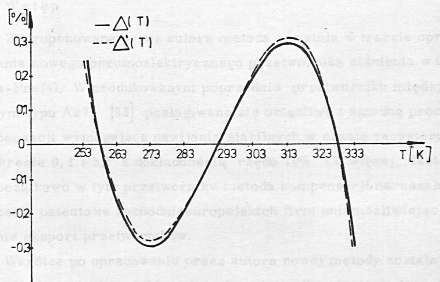
Considering Example 4 for $T_{o}$ = 293 K, $T_{1}$ = 258 K, $T_{2}$ = 328 K and $\Delta_{1}(T) = 2.5 \cdot 10^{-3} \cdot (T - 293)$ (i.e. a span drift of -2.5 %/10 K), using relation (63) we obtain:³

\Delta'(T) = -1.8 \cdot 10^{-5} \cdot (T-293) \cdot (T-288) \cdot (T-218) \cdot \left[ 1 + 2.5 \cdot 10^{-3} \cdot (T-293) \right]

s. 78

The geometrical interpretation is given in Fig. 26. The effect of the changes of the supply voltage is small, since it is expressed by a quantity of second order of smallness.

Fig. 26. Example of the temperature drift of the transducer zero Δ(T) and the change of this drift under the introduction of span compensation.

Translator's notes

"multiple bridge" (Polish "mostek wielokrotny") is the author's own term for this chain of Wheatstone bridges in which the output diagonal of each bridge supplies the next; a chain of two is called a "double bridge" ("dwójmostek", "mostek dwukrotny") and a chain of three a "triple bridge" ("mostek trójkrotny"); a single stage is a "single bridge" ("mostek jednokrotny"). The "double bridge" of this thesis is unrelated to the Kelvin (Thomson) double bridge used for low-resistance measurement. ↩
the symbols $a_{1} \ldots a_{9}$ here are division ratios of the dividers in Fig. 25, not the slope constants $a_{j}$ of the component functions in Chapter 4. ↩
factors as printed. (T-288) and (T-218) match neither the compensation temperatures $T_{1}$ = 258 K and $T_{2}$ = 328 K given in the same sentence nor the factors of $\Delta(T)$ in Example 4; the intended values cannot be established, so the expression is left as in the original. ↩