6. APPLICATION OF THE NEW COMPENSATION METHOD IN A PIEZORESISTIVE PRESSURE TRANSDUCER

s. 79

6.1. Introduction

The method proposed by the author arose in the course of the development of a new pneumatic-to-electric pressure transducer at the Mera-Pnefal Industrial Automation Research and Development Centre (OBRAP). In the previously manufactured inter-system converter type A271 [33] a burdensome and laborious compensation procedure was used, requiring the winding of long-term stable resistors in the range 0.1 to 5 Ω with an accuracy of the order of 10 %. Moreover, the compensation method initially applied in that transducer infringed the patent claims of West European firms, practically preventing the export of the transducers.¹

Soon after the author had developed the new method, it was tested in the pneumatic-to-electric pressure transducer type A272, and then, after positive results of the prototype tests, by decision of the Technical Council it was introduced into series production at Mera-Pnefal. In 1978 the manufacture of a series of 1000 units of these transducers is planned.

In the remainder of this work there will be presented the required parameters of the transducer, the construction and properties of the pressure sensor, a design outline of the more interesting subassemblies of the transducer connected with the temperature compensation circuit, and finally some results of the tests of the prototypes of the pneumatic-to-electric transducer carried out by the Product Testing Laboratory of the Quality Control Department of the Mera-Pnefal Industrial Automation Enterprise and by the Mera-Pnefal Industrial Automation Research and Development Centre.

6.2. Required metrological parameters of the transducer.

a. The construction of the transducer should be based on the sensor discussed in Section 6.3. b. input signal 20 to 100 kPa c. output signal: one of those listed, according to the choice of the customer

s. 80

0 - 5 mA
0 - 20 mA
0 - 50 mA
4 - 20 mA
10 - 50 mA
1 - 5 V
0 - 10 V d. transfer characteristic - linear e. intrinsic error 0.4 % f. operating temperature range: standard version 273 K to 333 K special version 253 K to 333 K g. supply voltage 25 V $^{+0.5V}_{-1.5V}$ with a common negative rail²

6.3. Sensor

6.3.1. Construction

The pressure sensor is built on the basis of silicon strain gauges. The input pressure is converted by means of the bellows assembly (Fig. 27) into a force producing stresses in the strain-gauge beam. The beam is rigidly fixed at one end, while at the other it is coupled to the bellows assembly. Two silicon strain gauges are bonded to the strain-gauge beam, one on each side. Under the action of the input pressure this beam deflects, which causes compressive stresses to arise in the upper gauge TS2 and tensile stresses in the lower gauge TS1, as a result of which an increase in the resistance value (of approx. 5 %) of gauge TS1 and a decrease in the resistance value of gauge TS2 are obtained. The beam is protected from overload by the beam travel stop. The gauge leads are soldered to the terminal board, from which the sensor signal is then conveyed by wires to the electronic

s. 82

signal-conditioning circuit.

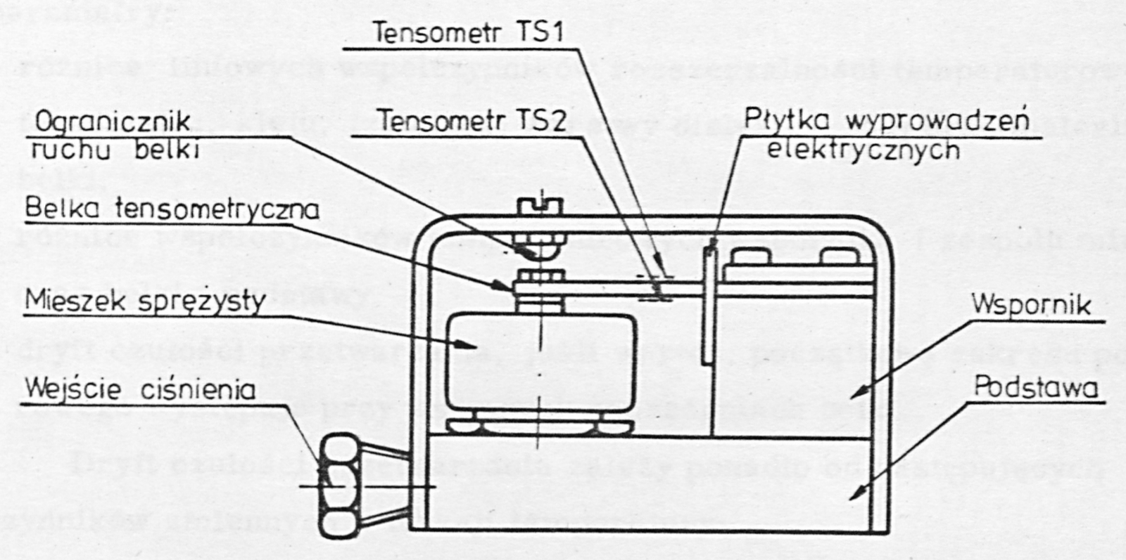
Labels: Tensometr TS1 = strain gauge TS1; Ogranicznik ruchu belki = beam travel stop; Tensometr TS2 = strain gauge TS2; Płytka wyprowadzeń elektrycznych = terminal board; Belka tensometryczna = strain-gauge beam; Mieszek sprężysty = bellows; Wspornik = bracket; Wejście ciśnienia = pressure inlet; Podstawa = base

The basic technical data of the sensor are: a. initial resistance of the gauges at a temperature of 293 K, at atmospheric pressure - 110 Ω ±11 Ω, b. spread of resistance of the gauges on one sensing beam 0 to 5 Ω, the gauge in tension having the greater resistance, c. full-scale resistance change of the gauges (for a change of pressure from 20 kPa to 100 kPa) - 5.6 Ω to 7.6 Ω.

6.3.2. Sources of temperature errors.

The basic source of the temperature errors of the sensor is the strain gauges. Both the initial resistance and the sensitivity of the gauges change strongly with temperature. The change of the initial resistance at atmospheric pressure (without stress) as a function of temperature for the gauges used has the character of a second-order curve. The sensitivity is determined by the relation:

s. 83

where: $c_{1}$, $c_{2}$ - constants

An additional influence on the drift of the lower range value is exerted by the following parameters:

• differences between the linear coefficients of thermal expansion of the gauge, the adhesive, the insulating dielectric layer and the beam material,
• differences between the temperature coefficients of the bracket and the bellows assembly, and of the beam and the base,
• the sensitivity drift, if the lower range value occurs with the beam under preload. The sensitivity drift depends moreover on the following factors that vary as a function of temperature:
• the effective area of the bellows and its compliance
• the Young's modulus of the strain-gauge beam
• the thickness of the layers insulating the gauges from the beam.

6.3.3. Selection of the parameters of the temperature compensation circuit

In order to obtain information on the temperature errors of the sensor, temperature-pressure tests of 16 pressure sensors were carried out in the measuring setup shown in Fig. 28. The tests were carried out in the temperature range from 253 K to 333 K, every 20 K. At each of these temperatures the static characteristic was measured at five input pressures. The input pressure was measured with an Ashcroft digital pressure gauge with an accuracy of ±0.05 % on the 200 kPa measuring range. The output signal of the sensor was read on a Hewlett-Packard 3490A digital voltmeter, with an accuracy of ±0.03 %. After analysis of the measurement results it was found that the temperature drift of the nonlinearity remains at the level of 0.007 %/10 K, so that temperature compensation of this parameter is unnecessary. The following procedure for determining the temperature errors of the zero was applied:

s. 84

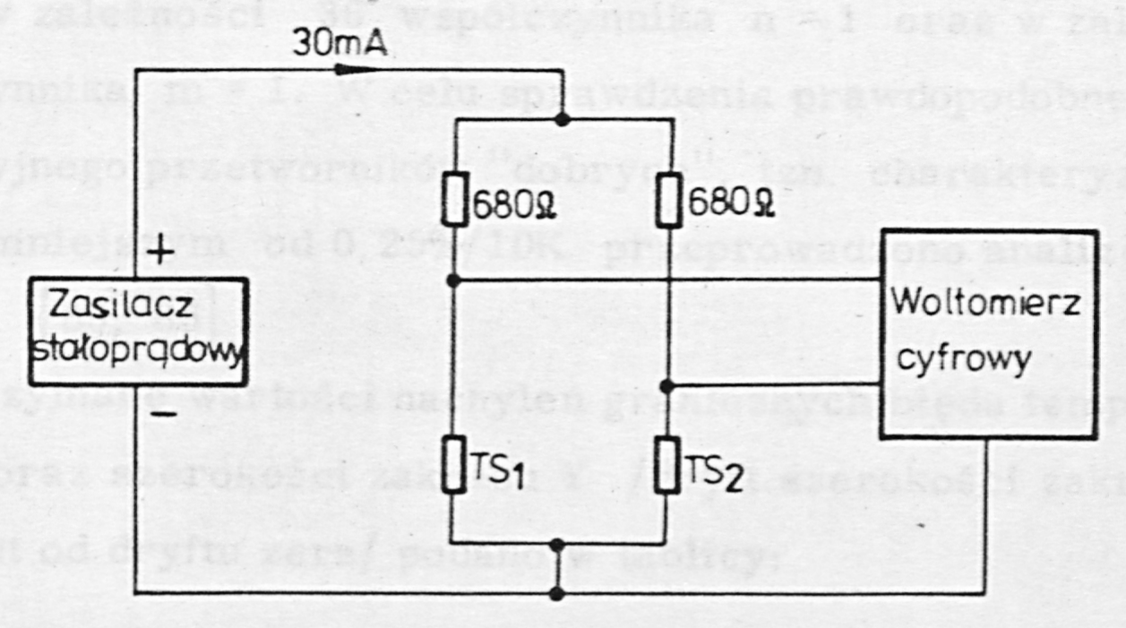
Labels: Zasilacz stałoprądowy = DC power supply; Woltomierz cyfrowy = digital voltmeter

a. for each of these parameters a straight line was drawn intersecting the plot of the sensor error at the temperatures 278 K (reference) and 308 K (first compensation), (Fig. 29a); b. the straight line was shifted parallel to itself so that it intersected the plot of the sensor error at the temperature 293 K (Fig. 29b); c. the maximum slope of the error with respect to this straight line was sought, determining the error limit according to PN-74/M-42020 (see Section 2, Fig. 2b.)

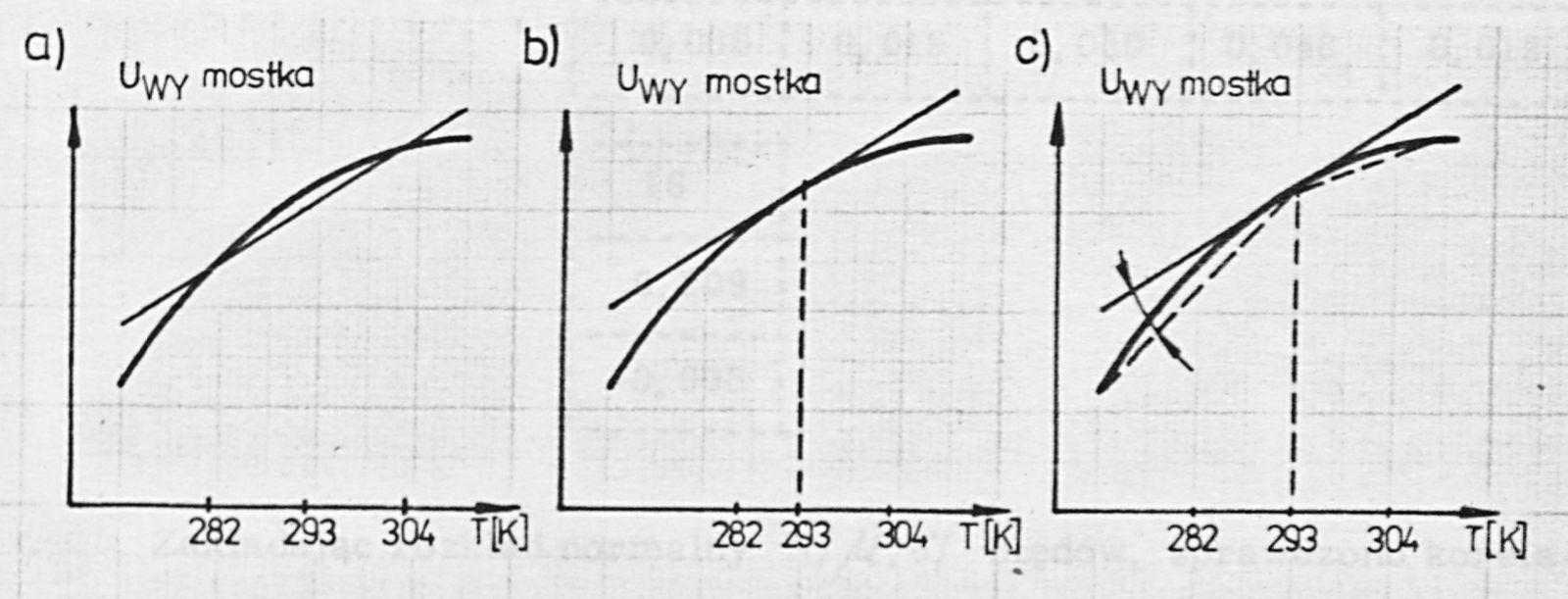
Labels: U_WY mostka = bridge output voltage

s. 85

The compensation procedure applied was equivalent to adopting in relation 36 the coefficient n = 1 and in relation 39 the coefficient m = 1. In order to check the probable production "yield" of "good" transducers, i.e. those characterized by an error smaller than 0.25 %/10 K, a statistical analysis of the results was carried out [83, 85].

The values obtained for the limiting slopes of the temperature error of the zero X and of the span Y (the span drift is made independent of the zero drift) are given in the table:

Sensor No.	X, %/10 K	Y, %/10 K
1	0.181	0.081
2	0.110	-0.033
3	0.176	0.013
4	0.051	0.074
5	0.083	-0.027
6	0.137	0.039
7	0.153	0.065
8	0.181	0.052
9	0.140	0.080
10	0.112	-0.015
11	0.175	0.086
12	0.183	0.019
13	0.144	0.050
14	0.134	0.048
15	0.192	0.012
16	0.209	-0.0053

Assuming a normal distribution $N(\mu, \sigma)$ of the errors, the correlation between the temperature drift of the zero and of the span was checked. The sample mean errors $\bar{X}$ and $\bar{Y}$ are

s. 86

whereas the sample standard deviations $S_{x}$ and $S_{y}$:

The correlation coefficient $r_{xy}$ is defined as follows:

where: n - the number of sensors $X_{i}$ - the value of the zero drift of the i-th sensor $Y_{i}$ - the value of the span drift of the i-th sensor

For the error values from Table 1 we obtain $r_{x,y}$ = 0.0162. Taking n = 16 and assuming a confidence level of 0.95, one obtains the confidence interval for the unknown true value of the correlation coefficient [-0.38, +0.6].⁴

Calculating the critical value of the correlation coefficient [85] we obtain

The value of the correlation coefficient observed in the sample batch of sensors, as determined by its confidence interval, is greater than the critical value, so there are no grounds for rejecting the hypothesis that the zero drift and the span drift are correlated with each other. Since, however, the value obtained for the correlation coefficient is small, it cannot be used as additional information on the sensor error in accordance with Section 4.3.3.

Observation of the scatter of the limiting zero and span drifts (Fig. 30) confirms this conclusion.

s. 87

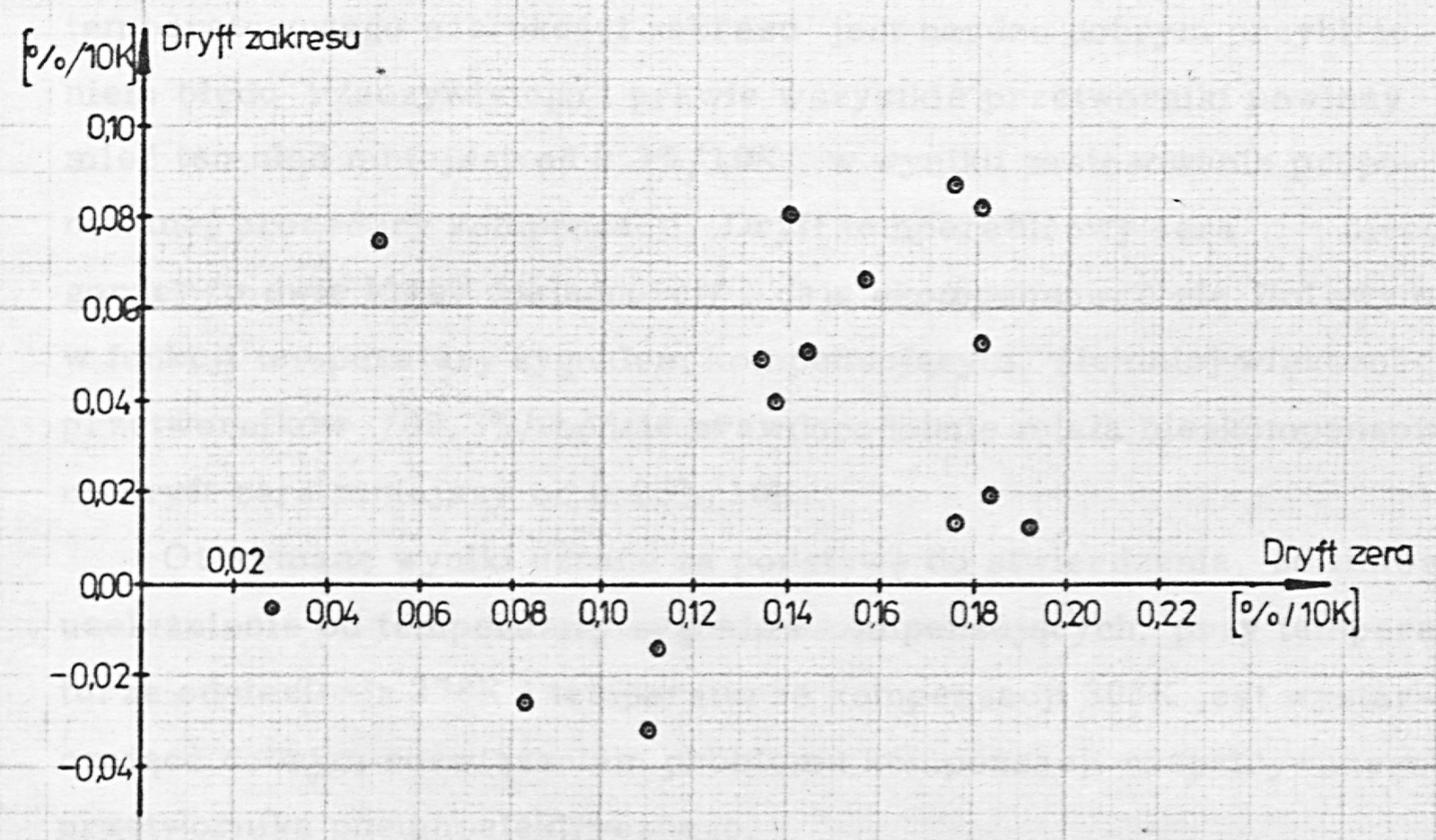
Labels: Dryft zakresu = span drift; Dryft zera = zero drift

Taking into account the values obtained for the mean error limits $\bar{X}$ and $\bar{Y}$ and the sample standard deviations, we may quantify the effects of applying the proposed temperature compensation procedure. Namely, we may calculate the probability of obtaining transducers with an uncompensated error smaller than: 0.05 %/10 K, 0.1 %/10 K, 0.16 %/10 K and 0.25 %/10 K. The results are presented in Table 2.

Table 2

A	0.05	0.1	0.16	0.25	%/10 K
$P(X<A)$	0.8	12.3	65.2	99.3	%
$P(Y<A)$	68.8	97.7	99.997	1	5

s. 88

From the above data it follows that the linear approximation of the temperature drift of the span is a very good approximation of the real error, and almost all transducers should have this error smaller than 0.1 %/10 K as a result of applying the proposed compensation procedure. The temperature drift of the zero lends itself somewhat less well (by two accuracy classes) to compensation by a compensating signal linear in temperature; nevertheless the majority of transducers (99.3 %) will probably have an uncompensated zero drift smaller than 0.25 %/10 K.

The results obtained were taken as the basis for stating that a linear temperature dependence of the compensating signals, with a reference temperature of 278 K and a compensation temperature of 308 K, is a sufficiently good solution of the compensation problem for the pneumatic-to-electric transducer under consideration.

6.4. Electronic circuit of the transducer

6.4.1. Block diagram

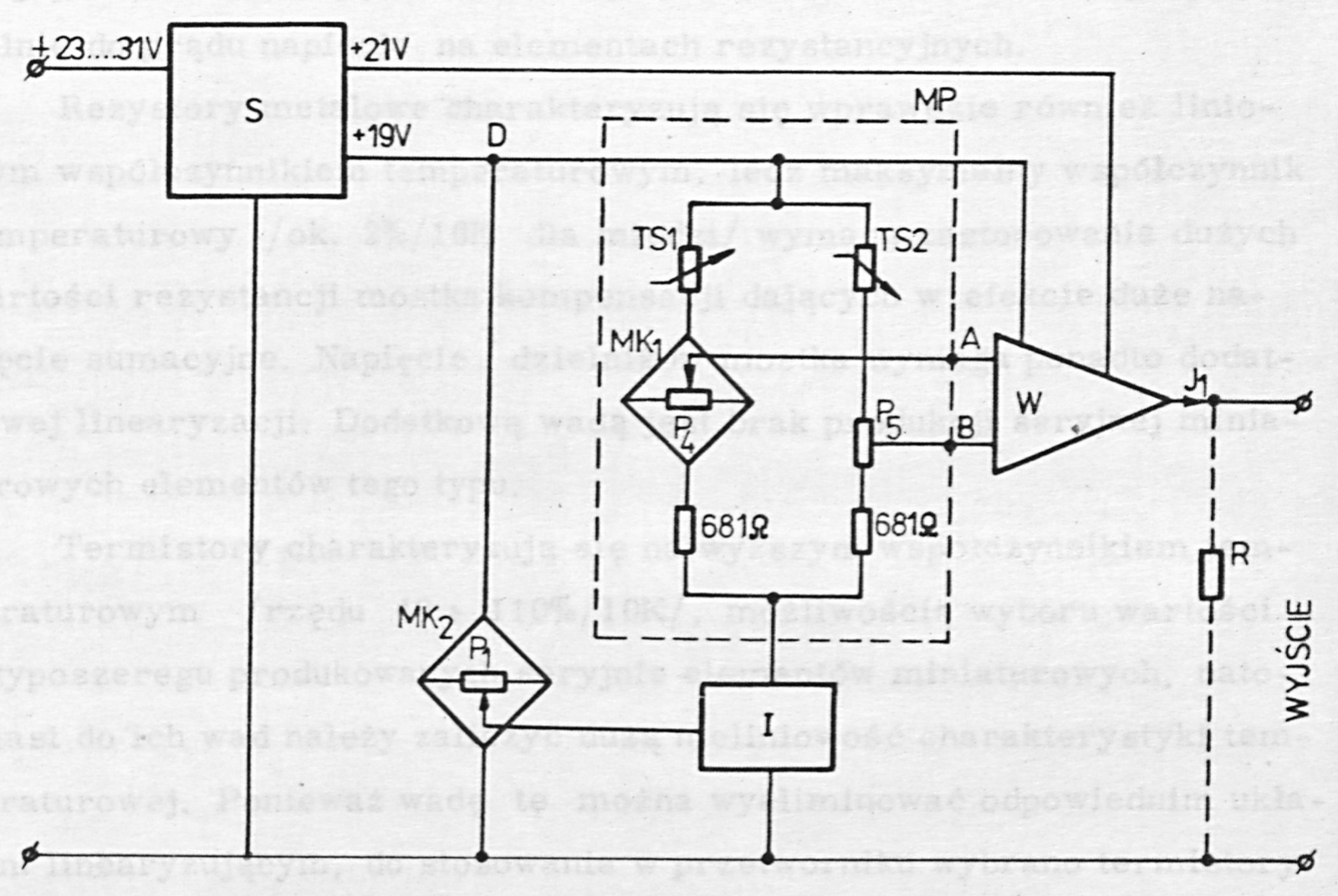
The block diagram of the transducer circuit design chosen by the author [87] is shown in Fig. 31. The transducer is built of six main assemblies

• the measuring bridge MP
• the single bridge $MK_{1}$ for the temperature compensation of the lower range value
• the voltage-difference-to-current converter W
• the current source I
• the single bridge $MK_{2}$ for the temperature compensation of the upper range value (span)
• the regulated power supply

The measuring bridge makes it possible to convert the change of resistance of the strain gauges TS into a change of voltage on the bridge diagonal. At the same time, as a result of the differential connection of the gauges, a preliminary compensation of the effect of temperature is realized. In addition the circuit makes it possible to null the voltage on the bridge diagonal at the lower range value and

s. 89

to add to the voltage signal from the gauges the voltage of the generator of the zero temperature-compensation signal, in the form of the single bridge $MK_{1}$.

The single bridge $MK_{1}$ makes it possible to null the measuring bridge at the reference temperature independently of the setting of potentiometer $P_{4}$, because on this potentiometer, connected across the diagonal of the compensation bridge $MK_{1}$, there is zero voltage at the reference temperature. At the compensation temperature a voltage is produced on potentiometer $P_{4}$, a part of which, set by the position of the potentiometer wiper, is used to null the measuring bridge again, i.e. to compensate the temperature drift of the lower range value.

The measuring bridge is supplied by the current source I. The source current of this source is controlled by the potential of the wiper of potentiometer $P_{1}$, placed on the diagonal of the single bridge $MK_{2}$. At the reference temperature there is zero voltage on this potentiometer and the source current is determined by the value of the potential of the end terminals of the potentiometer, independently of the position of its wiper. At the first compensation temperature a certain voltage is produced on the potentiometer, and consequently a change in the position of the potentiometer wiper changes the value of the current supplying the measuring bridge, which is used to compensate the temperature error of the upper range value.

The differential signal from the diagonal of the measuring bridge MP is converted by the circuit W, with an adjustable conversion factor, into the output current $I_{1}$. To produce the voltage output signal of the transducer there serves a resistor R shunting the output terminals.

The voltage regulator S supplies two supply voltages:

• the internal supply reference voltage +19 V
• the auxiliary voltage for supplying the transducer circuit +21 V

The whole circuit is supplied from a single voltage with a nominal value of 25 V.

s. 90

Labels: WYJŚCIE = output (wyjście)

6.4.2. Choice of the temperature-sensing elements

The following components were considered as temperature-sensing elements:

• diodes
• transistors
• metal resistors
• thermistors

Diodes and transistors are characterized both by a large temperature coefficient of the forward or base-emitter voltage (approx. 3 %/10 K) and by a highly linear change of this voltage over a wide temperature range. Among the basic drawbacks of these components must be counted the large spread of the value of this voltage when discrete components are used, of the order of the full-scale signal of the sensor. Moreover, their use would increase the common-mode voltage of the sensor by several hundred

s. 91

millivolts. An additional argument that influenced the rejection of these components is the fact that if, in the state of bridge balance, the supply current were to change, this would cause bridge unbalance on account of the stabilizing characteristics of these components and of the voltage on the resistive components being proportional to the current.

Metal resistors, it is true, are also characterized by a linear temperature coefficient, but the maximum temperature coefficient (approx. 2 %/10 K for copper) requires the use of large values of resistance in the compensation bridge, giving in effect a large common-mode voltage. The voltage of the bridge dividers moreover requires additional linearization. An additional drawback is the absence of series production of miniature components of this type.

Thermistors are characterized by the highest temperature coefficient (of the order of 40 to 110 %/10 K), by the possibility of choosing the value from the standard value series of series-produced miniature components, whereas among their drawbacks must be counted the large nonlinearity of the temperature characteristic. Since this drawback can be eliminated by a suitable linearizing circuit, thermistors were chosen for use in the transducer. In the remainder of this work the circuits linearizing the characteristics of the thermistors are presented.

s. 92

6.4.3. Optimization of the characteristics of the bridge compensating the zero drift

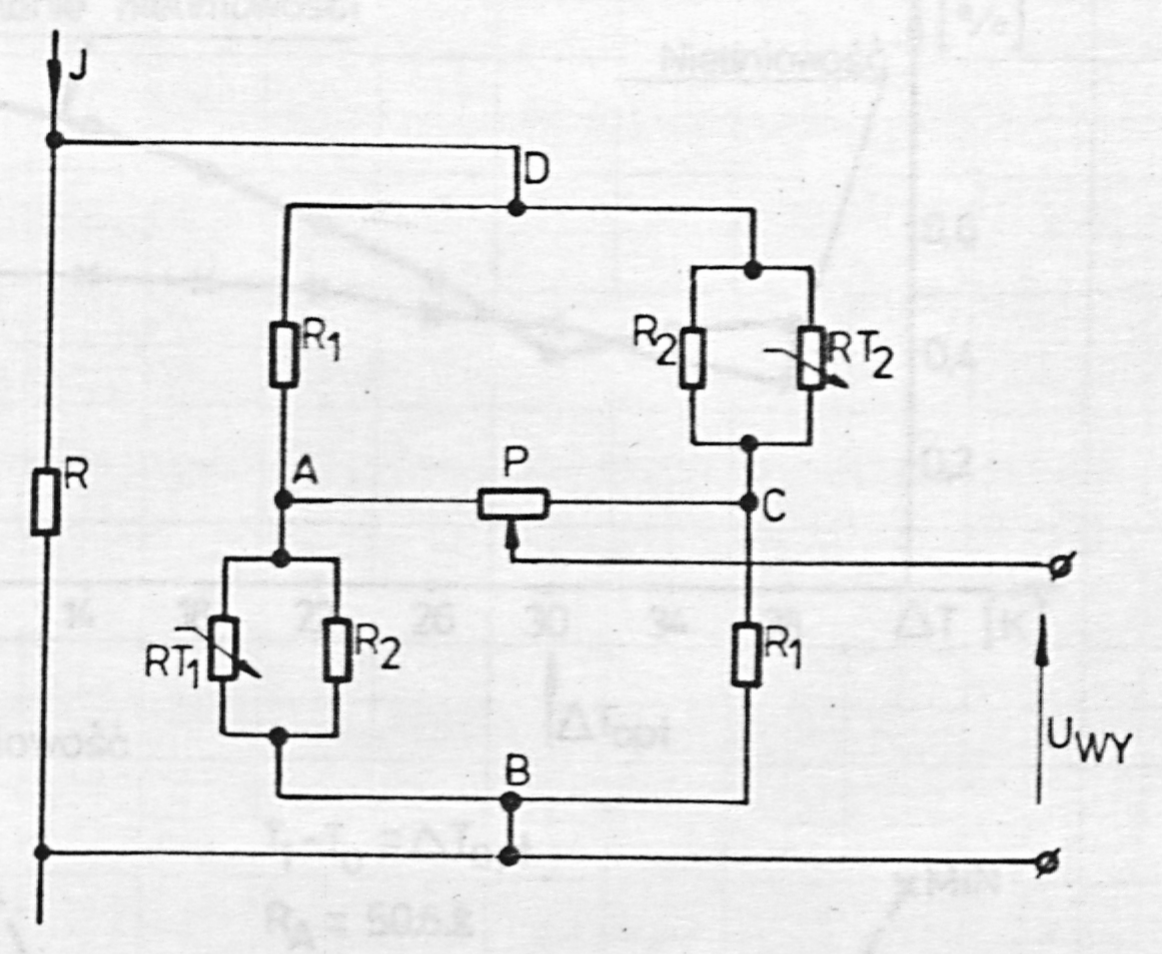
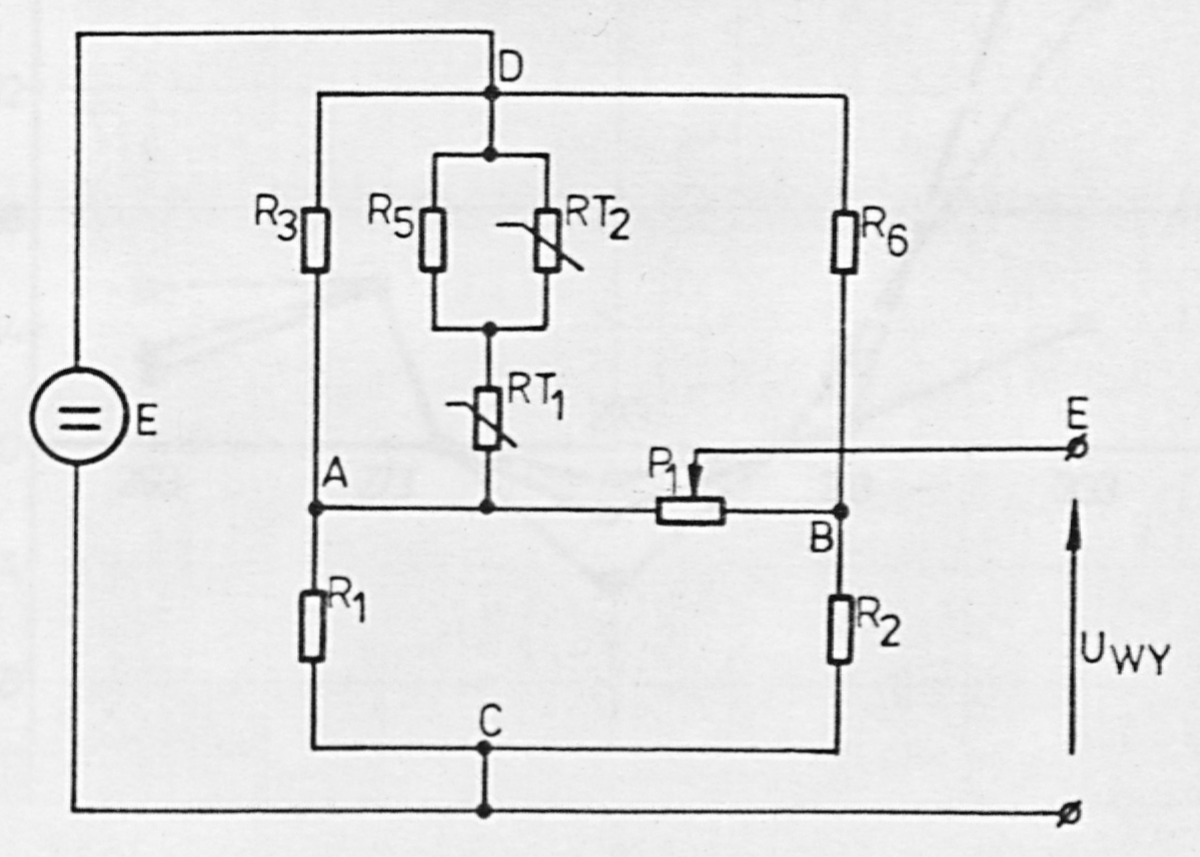
The circuit of the bridge compensating the temperature drift of the zero should provide a linear change of voltage with changes of temperature, adjustable in the range from -8 %/80 K to +8 %/80 K. It was decided to check the circuit of a single-thermistor voltage divider with regard to the possibility of obtaining a voltage on the bridge arms that is suitably linear as a function of temperature (Fig. 32). The bridge is built of two such dividers connected in opposition. As a result the voltage $U_{AB}$ decreases, whereas the voltage $U_{CB}$ increases with temperature.

In order to reduce the effect of changes of the bridge resistance on the voltage $U_{DB}$ under constant-current excitation, a shunt resistor R was introduced.

For the linearization of the voltages $U_{AB}$ and $U_{CB}$ as a function of temperature, use was made of the nonlinear relation determining the value of the resultant resistance of the resistor $R_{2}$ and the thermistor RT connected in parallel, and of the nonlinear relation determining the division ratio of the resistive divider $R_{1}$ - $R_{2}$/RT.

The optimum values of the resistors $R_{1}$, $R_{2}$ were calculated by means of a computer program. The calculations were carried out for 8 pairs of temperatures (reference temperature $T_{o}$ - compensation temperature $T_{1}$), starting from 288 K - 298 K and ending at 274 K - 312 K, where at each successive step both temperatures were changed simultaneously by 2 K. The optimization consisted in minimizing the slope of the nonlinearity of the divider with respect to the temperature 293 K.

A thermistor of type NTC110 with a nominal resistance of 47 Ω at a temperature of 298 K was used here. The characteristics of the thermistors were determined experimentally by measuring the resistance values in the temperature range 253 K to 333 K every 20 K. A lack of agreement was found between the resistance of the thermistors in the measured temperature range and the generally accepted approximation RT = Aexp(B/T). Since, however, this approximation was sufficiently accurate over an interval of 20 K, for determining the resistance of the thermistors at the compensation temperatures $T_{1}$ and reference temperatures $T_{o}$ the above relation was used, the constants A and B being determined on the

s. 93

Labels: U_WY = output voltage (WY = wyjście, output)

basis of the resistance values of the thermistor at the neighbouring temperatures.

On the basis of the measurement results for 6 thermistors the mean characteristic was determined, and the optimization was carried out for this characteristic; the nonlinearity as a function of temperature was then checked for the mean characteristic and for the extreme characteristics of the thermistors, i.e. the maximum and minimum characteristics.

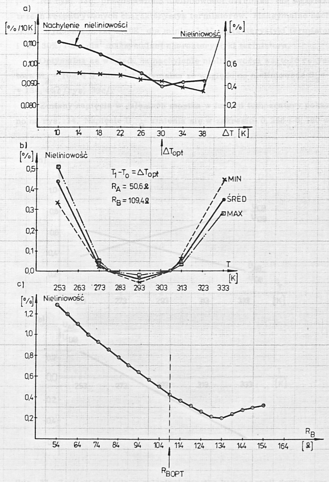
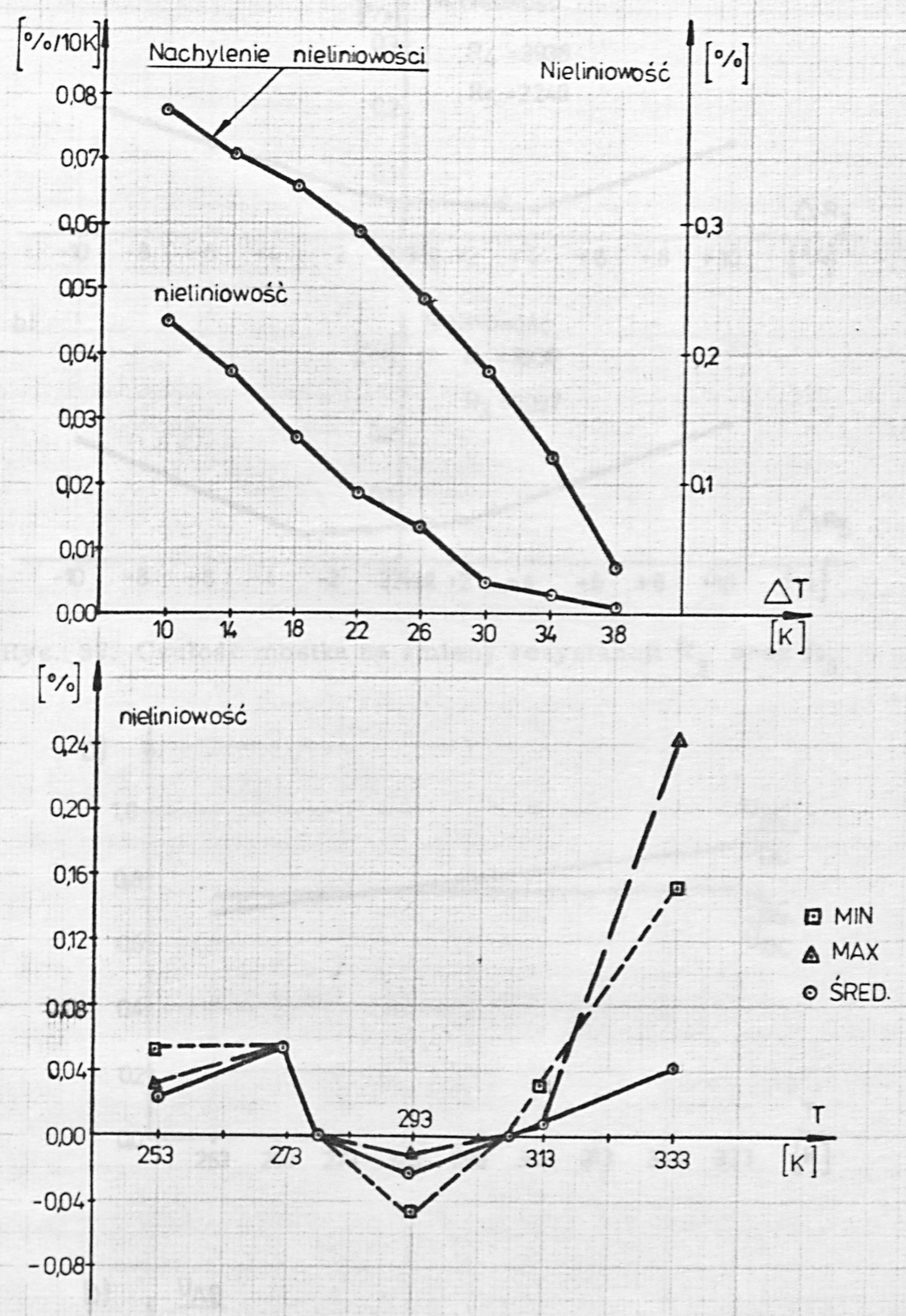
The results of the calculations are presented in Fig. 33. The minimum value of the slope M, equal to 0.089 %/10 K, was obtained for the pair of temperatures $T_{o}$ = 278 K, $T_{1}$ = 308 K (Fig. 33a.) The smallest value of the nonlinearity (the difference D) was obtained for the pair of temperatures 274 K - 312 K. Since in accordance with PN-74/M-42020 it is the slope of the error that is assessed, it was decided to choose the reference temperature $T_{o}$ = 278 K and the compensation temperature $T_{1}$ = 308 K.

At these temperatures the optimum resistor values $R_{1}$ = 50.6 Ω and $R_{2}$ = 109.4 Ω provide a change of the division ratio of 42.2 % for a change of temperature from 253 K to 333 K.

s. 94

Labels: Nachylenie nieliniowości = slope of the nonlinearity; Nieliniowość = nonlinearity; ŚRED = mean (abbreviation of średnia)

s. 95

Fig. 33b shows the nonlinearities of the divider for all three thermistor characteristics considered. The maximum slopes are: 0.125 %/10 K for the minimum thermistor characteristic and 0.130 %/10 K for the maximum thermistor characteristic.

The value of the resistor $R_{2}$ = 109.4 Ω that is optimum with respect to the slope of the nonlinearity is not optimum with respect to the nonlinearity, $R_{2}$ = 134.4 Ω (Fig. 33c).

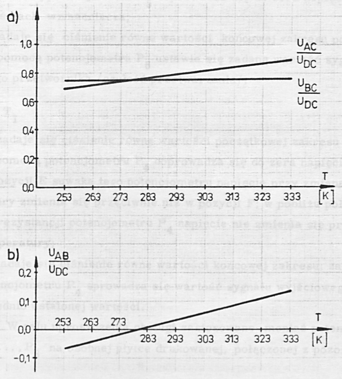
The changes of voltage in the bridge arms as a function of temperature are shown in Fig. 34. The voltage $U_{CB}$ varies in the range 0.368 to 0.790 of the

s. 96

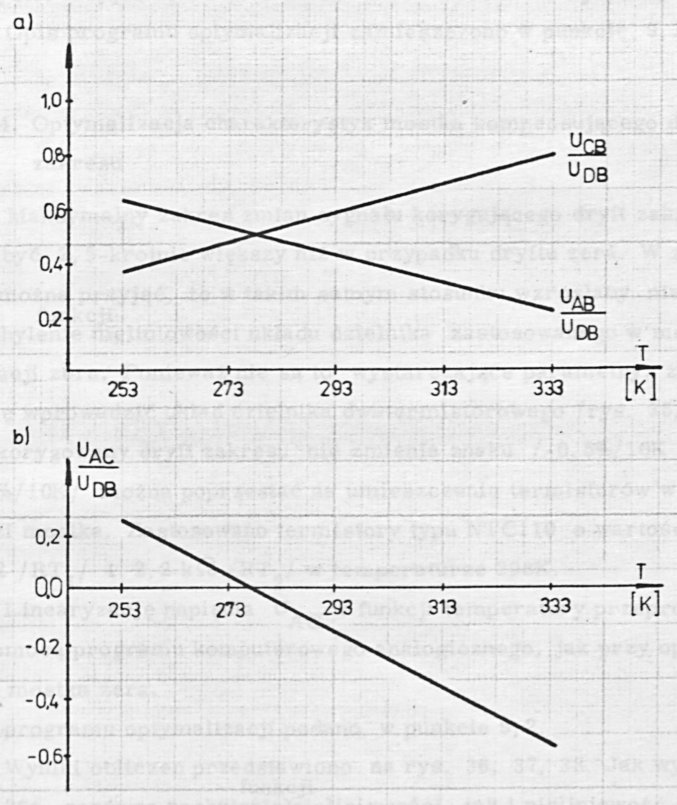
value of the voltage $U_{DB}$ supplying the bridge, whereas the voltage $U_{AB}$ varies in the range 0.532 to 0.210 of the value of the voltage $U_{DB}$ (Fig. 34a). The voltage $U_{AC}$ occurring on the potentiometer varies in the range from +0.264 to -0.580 of the value of the voltage $U_{DB}$ (Fig. 34b).

From the results presented in Fig. 33b it follows that the maximum slope of the nonlinearity function is caused by the large nonlinearity occurring at the extreme temperatures. In the temperature range 273 K to 313 K the value of this slope is more than two times smaller.⁶

In view of the fact that the maximum zero drift of the sensors (1 %/10 K) is two times greater than the mean drift, the results obtained were considered sufficiently good for use in the zero compensation bridge.

A description of the optimization program is given in Section 9.1.⁷

6.4.4. Optimization of the characteristics of the bridge compensating the span drift

The maximum range of variation of the signal correcting the span drift should be 2.5 times greater than in the case of the zero drift. In connection with this it may be assumed that the nonlinearity and the slope of the nonlinearity function of the divider circuit used in the zero compensation bridge would increase in the same ratio. Since these are not sufficient parameters, it was decided to introduce a two-thermistor divider circuit (Fig. 35). Since the span drift being corrected does not change sign (-0.5 %/10 K to -2.5 %/10 K), it is enough to place the thermistors in one arm of the bridge. Thermistors of type NTC110 with values of 680 Ω ($RT_{1}$) and 2.2 kΩ ($RT_{2}$) at a temperature of 298 K were used.

The linearization of the voltage $U_{AC}$ as a function of temperature was carried out by means of a computer program analogous to that used in the optimization of the zero bridge. A description of the optimization program is given in Section 9.2.

The results of the calculations are presented in Figs. 36, 37, 38. As follows from Fig. 36a, both the slope of the nonlinearity function and the nonlinearity are (after allowing for the increased range of variation of the division ratio) an order of magnitude smaller than in the single-thermistor circuit.

s. 97

Both of these parameters are the smaller, the greater the difference between the reference and compensation temperatures. Sufficiently good results are obtained for the pair of temperatures $T_{o}$ = 278 K, $T_{1}$ = 308 K, at which the minimum of the slope of the nonlinearity function in the zero compensation bridge occurs.

The nonlinearity as a function of temperature for this pair of temperatures is shown in Fig. 36b. The maximum slope of the nonlinearity function is 0.038 %/10 K for the mean thermistor characteristic, and 0.050 %/10 K for the minimum characteristic and 0.063 %/10 K for the maximum characteristic. Considering that the mean value of the span drift is almost two times smaller than the maximum value, the results obtained must be regarded as entirely satisfactory.

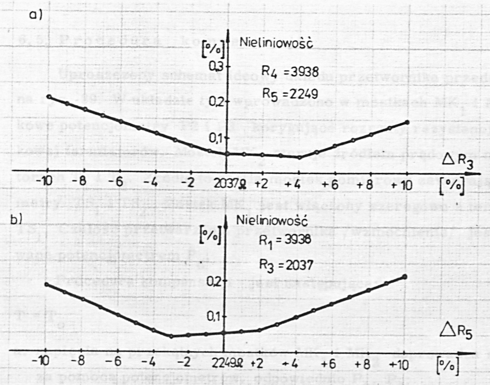
The sensitivity of the circuit to changes in the values of the resistors $R_{3}$ and $R_{5}$ is shown in Fig. 37 a and b. One may note the occurrence of a minimum nonlinearity for a value of resistor $R_{3}$ 4 % greater, and for a value of resistor $R_{5}$ 3 % smaller, than the respective values guaranteeing the minimum value of the slope of the nonlinearity function.

The temperature characteristic of the bridge is given in Fig. 37a, and the voltage on potentiometer $P_{1}$ in Fig. 36b.⁸

Labels: U_WY (WY = wyjście) = U_out (output voltage)

s. 98

Labels: Nachylenie nieliniowości = slope of the nonlinearity; Nieliniowość = nonlinearity; ŚRED. = mean

s. 99

Labels: Nieliniowość = nonlinearity

s. 100

6.5. Compensation procedure

A simplified circuit diagram of the transducer circuit is shown in Fig. 39. In this circuit additional potentiometers P2 and P3, correcting the spread of the initial resistance of the thermistors, have been introduced into the bridges $MK_{1}$ and $MK_{2}$. The bridge $MK_{2}$ controls the current source on the transistors $T_{1}$ and $T_{2}$. This source supplies the measuring bridge containing the strain gauges $TS_{1}$ and $TS_{2}$. The bridge $MK_{1}$ is connected in series with the strain gauge $TS_{1}$. The sensitivity of the transducer (gain) is adjusted by potentiometer $P_{6}$.^{9 10}

The compensation procedure is as follows:

T = $T_{o}$

a. the voltages on the diagonals of the bridges $MK_{1}$ and $MK_{2}$ are brought to zero by means of potentiometers $P_{3}$, $P_{2}$ respectively; b. a pressure equal to the lower range value is applied; by means of potentiometer $P_{5}$ the voltage $U_{GH}$ at the amplifier inputs is brought to zero; c. a pressure equal to the upper range value is applied; by means of potentiometer $P_{6}$ the required value of the transducer output signal (sensitivity) is set;

T = $T_{1}$

a. a pressure equal to the lower range value is applied; by means of potentiometer $P_{4}$ the voltage $U_{GH}$ is brought to zero; in position E of the wiper of this potentiometer the voltage changes with changes of temperature in the opposite sense to that in position F; near the middle of the resistance value of potentiometer $P_{4}$ the voltage does not change with a change of temperature; b. a pressure equal to the upper range value is applied; by means of potentiometer $P_{1}$ the value of the output signal is brought to the value established previously.¹¹

In order to simplify handling, the potentiometers $P_{1}$,...,$P_{6}$ are mounted on a separate printed-circuit board, connected to the rest of the

s. 101

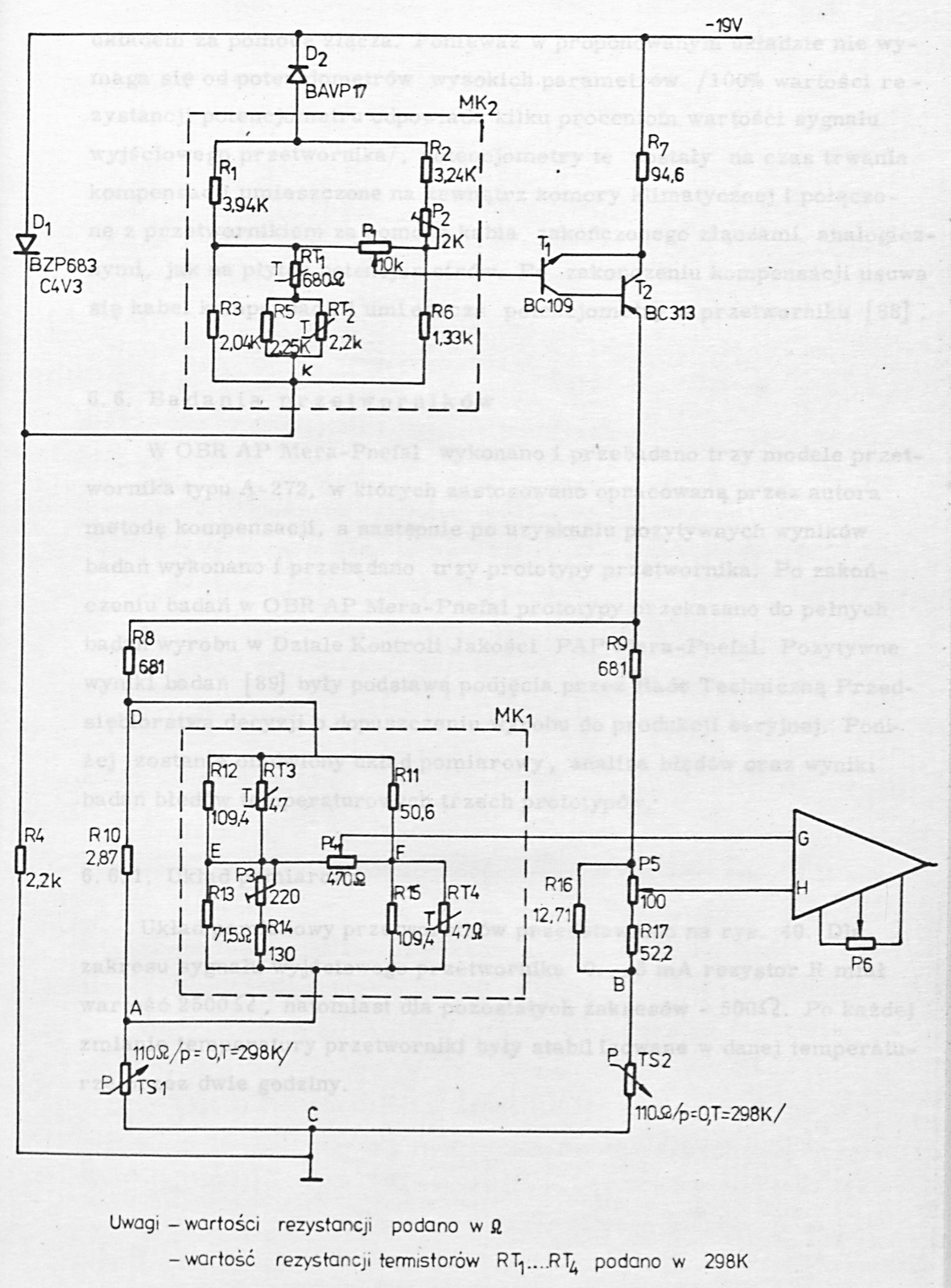
Labels: Uwagi = notes; wartości rezystancji podano w Ω = resistance values are given in Ω; wartość rezystancji termistorów RT1…RT4 podano w 298K = the resistance of thermistors RT1…RT4 is given at 298 K

s. 102

circuit by means of a connector. Since in the proposed circuit high performance is not required of the potentiometers (100 % of the resistance value of the potentiometer corresponds to a few per cent of the value of the transducer output signal), these potentiometers were placed, for the duration of the compensation, outside the climatic chamber and connected to the transducer by means of a cable terminated with connectors analogous to those on the potentiometer board. After completion of the compensation the compensation cable is removed and the potentiometers are placed in the transducer [88].

6.6. Transducer tests

At the Mera-Pnefal Industrial Automation Research and Development Centre (OBR AP) three engineering models of the transducer type A-272 were made and tested, in which the compensation method developed by the author was applied, and then, after positive test results had been obtained, three prototypes of the transducer were made and tested. After completion of the tests at OBR AP Mera-Pnefal the prototypes were handed over for full product tests at the Quality Control Department of the Mera-Pnefal Industrial Automation Enterprise (PAP). The positive test results [89] were the basis for the decision of the Technical Council of the enterprise to release the product for series production. Below are discussed the measuring setup, the error analysis and the results of the tests of the temperature errors of the three prototypes.

6.6.1. Measuring setup

The measuring setup for the transducers is shown in Fig. 40. For the transducer output signal range 0 to 5 mA the resistor R had a value of 2500 Ω, and for the remaining ranges 500 Ω. After each change of temperature the transducers were allowed to stabilize at the given temperature for two hours.

s. 103

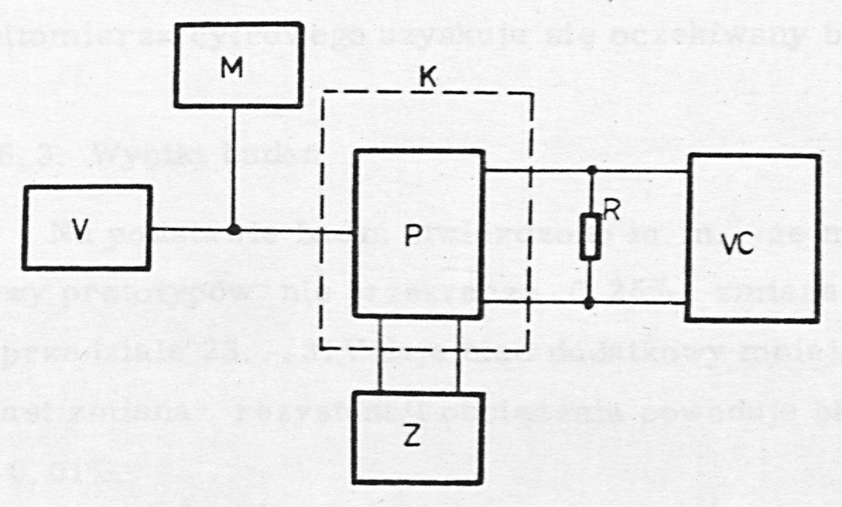
• P - transducer under test
• R - standard resistor 500 Ω or 2500 Ω, accuracy ±0.02 %
• VC - digital voltmeter type 3490A, Hewlett Packard
• Z - power supply V-316, Meratronik
• M - digital pressure gauge, Ashcroft, type 7781
• V - precision pressure setter
• K - variable-temperature chamber

6.6.2. Error analysis

The digital pressure gauge used for measuring the input pressure is characterized by a measuring range of 200 kPa and an accuracy of ±0.05 % of the measuring range. Transferring this accuracy to the measuring range of the transducer, 20 to 100 kPa, one obtains an accuracy of 0.125 % of the measuring range of the transducer (80 kPa).

The transducers tested had the following output signal values: 0 to 5 mA, 0 to 20 mA and 4 to 20 mA. The output signal was measured by measuring the voltage on the standard resistor, 500 Ω or 2500 Ω ±0.02 %, by means of a digital voltmeter with a 120 000-count display. In all cases a measured output voltage range of 10 V was obtained. The accuracy of the measurement made with the digital voltmeter was better than 0.01 % of the measured range

s. 104

Taking into account the errors of the pressure gauge, of the manufacture of the resistors R and of the digital voltmeter, one obtains an expected measurement error d = 0.073 %

6.6.3. Test results

On the basis of the tests it was found, among other things, that the maximum intrinsic error of the prototypes does not exceed 0.25 %, a change of the supply voltage in the interval 23 to 31 V gives an additional error smaller than 0.04 %, whereas a change of the load resistance causes an additional error smaller than 0.01 %.¹²

The temperature error was determined in the test report [89] with the intrinsic error included. As the temperature error of the transducer was taken the greatest slope of the changes of the transducer output signal at 20 kPa or 100 kPa with respect to the temperature 293 K. With this interpretation the following maximum temperature errors were obtained:

• for the transducer with the 0 to 5 mA range - 0.193 %/10 K
• for the transducer with the 0 to 20 mA range - 0.128 %/10 K
• for the transducer with the 4 to 20 mA range - 0.050 %/10 K

In the tests carried out at OBR AP Mera-Pnefal, in determining the temperature error the intrinsic error was disregarded, and only the change of the output signal for the zero (20 kPa) and for the span (80 kPa) caused by the change of temperature was taken into account. The tests were carried out at seven temperatures in the range from 253 K to 333 K. The test results are presented in Figs. 41, 42, 43. The dashed line shows the temperature error limit. It amounts to

• for the transducer with the 0 to 5 mA range - limiting zero drift 0.02 %/10 K, limiting span drift 0.14 %/10 K
• for the transducer with the 0 to 20 mA range - limiting zero drift 0.07 %/10 K, limiting span drift 0.11 %/10 K
• for the transducer with the 4 to 20 mA range - limiting zero drift 0.06 %/10 K, limiting span drift 0.09 %/10 K

s. 105

s. 106

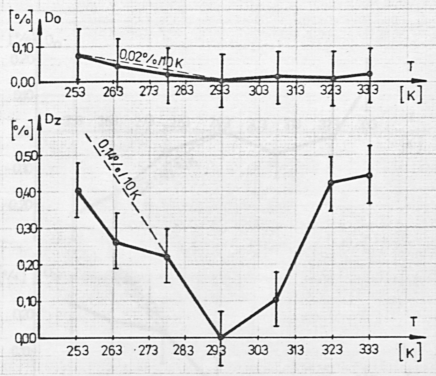
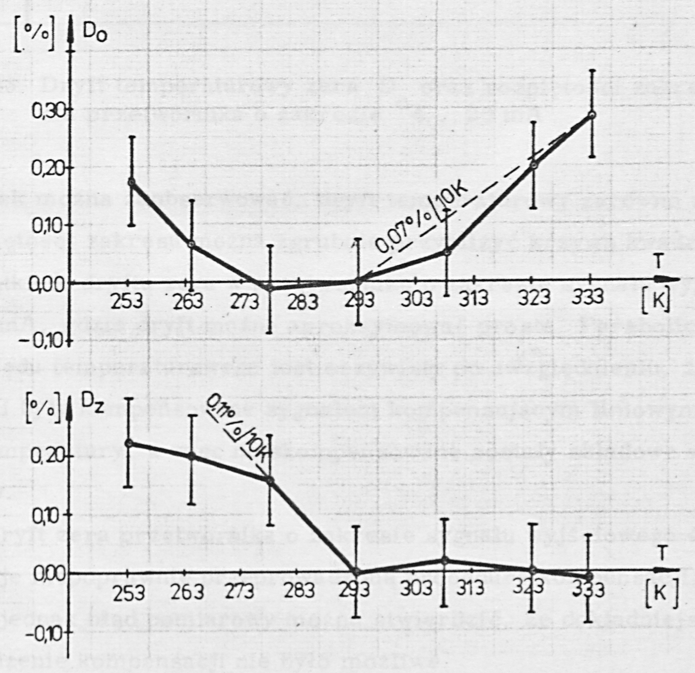
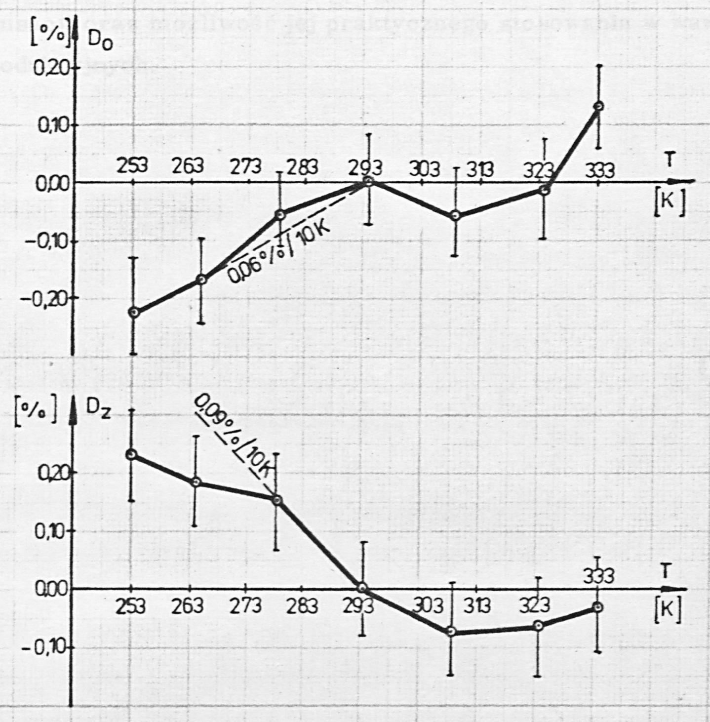
As may be observed, the temperature drift of both the zero and the span can be coarsely approximated by a quadratic curve, with the exception of the zero drift in the transducer with the 4 to 20 mA output signal range, where the drift can be approximated by a straight line. The parabolic course of the temperature error is obvious once it is taken into account that the transducers were compensated with a compensating signal linear in temperature, so that the higher-order components were left uncompensated. The zero drift of the transducer with the 4 to 20 mA output signal range suggests an incorrectly performed compensation procedure. Taking the measurement error into account, however, it can be stated that a more accurate performance of the compensation was not possible.

s. 107

The test results fully confirm the effectiveness of the new compensation method and the possibility of its practical application under production conditions.