4. A NEW METHOD OF COMPENSATION OF TEMPERATURE ERRORS

4.1. Introductory remarks

The new method of compensation of temperature errors proposed below [81, 82] eliminates the drawbacks of the known methods, while at the same time making it possible to reduce the temperature error of the transducer identically to zero.

In order to make the considerations presented below unambiguous, restrictions will be stated for the class of transducers whose compensation will be analysed: (a) the subject of the considerations will be transducers with a linear transfer characteristic from pressure to an electrical signal, (b) it is assumed that the only source of the temperature errors of the transducer is the sensor. If it is required to take into account the temperature drifts of other units of the transducer located at the same temperature as the sensor (e.g. the electronic signal-conditioning circuit), they should be referred to the level of the sensor, and the equivalent sensor error (in the sense of Section 2 of this thesis) should be subject to compensation, (c) additivity of the value of the measured parameter and of the value of the temperature error is assumed, i.e. it is assumed that the value of the parameter under consideration at an arbitrary temperature is described by the sum of the value of the parameter at the reference temperature and the temperature error, (d) the subject of the considerations will be errors in temperature steady states; the effect of temperature in the transient state will not be analysed, because this error is inseparably linked with the design of the transducer.

s. 39

4.2. Sufficient conditions for the temperature compensation of the transfer characteristic of the transducer

Let the transfer characteristic (2) of the transducer be described by a linear relation (Fig. 14):

U = U_{p} + \alpha_{1} X \qquad (3)

where: $U_{p}$ - the lower range value of the transducer output signal, at the lower range value $X_{p}$ of the non-electrical quantity $\alpha_{1}$ - the sensitivity¹

The changes of the output signal under the effect of temperature are determined by the partial differential equation

\frac{\partial U}{\partial T} = \frac{\partial U_{p}}{\partial T} + X \frac{\partial \alpha_{1}}{\partial T} \qquad (4)

In order to satisfy the condition of complete temperature compensation of the output signal

\frac{\partial U}{\partial T} = 0 \qquad (5)

two solutions of equation (4) are obtained

\frac{\partial U_{p}}{\partial T} = - X \frac{\partial \alpha_{1}}{\partial T} \qquad (6)

\left\{ \begin{aligned} \frac{\partial U_{p}}{\partial T} &= 0 \\ \frac{\partial \alpha_{1}}{\partial T} &= 0 \end{aligned} \right. \qquad (7)

s. 40

Fig. 14. Transfer characteristic of the transducer

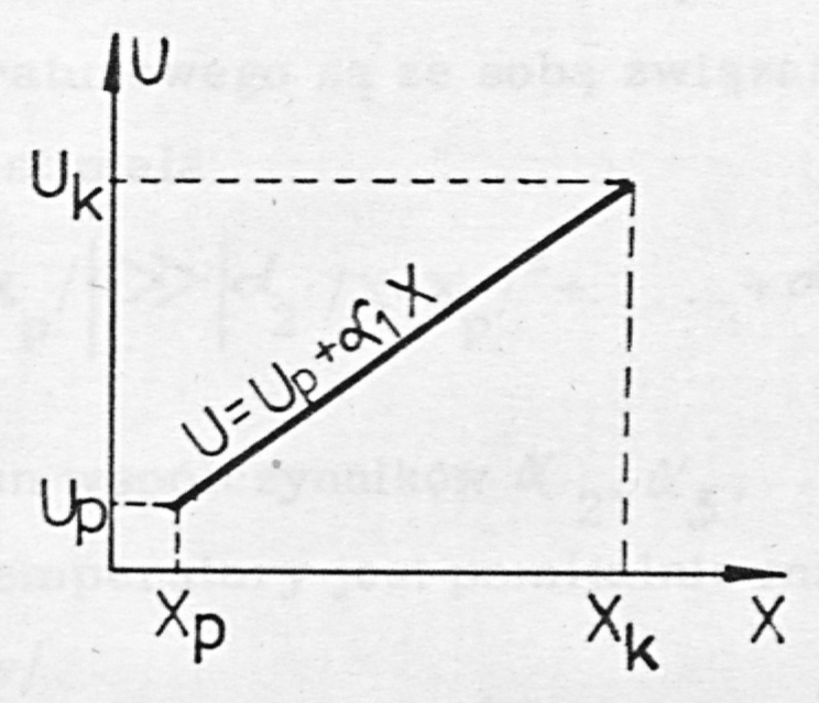
Condition a. has no practical significance, because of the changes as a function of the measured value of pressure.

The temperature compensation of most measuring transducers is based on condition b., which we may define as follows:

A sufficient condition for the temperature compensation of the transfer characteristic (3) is making the lower range value $U_{p}$ and the sensitivity $\alpha_{1}$ independent of temperature. We may modify this condition: for the temperature compensation of the transfer characteristic (3) it is sufficient to make the lower range value $U_{p}$ and the upper range value $U_{k}$ of the measuring range of the transducer independent of temperature. This is obvious, since the upper range value $U_{k}$ is a function of the lower range value and of the sensitivity:

U_{k} = U_{p} + \alpha_{1} (X_{k} - X_{p}) \qquad (8)

In reality the transfer characteristic also exhibits a certain nonlinearity ¹

U = U_{p} + \alpha_{1} (X - X_{p}) + \alpha_{2} (X - X_{p})^{2} + \alpha_{3} (X - X_{p})^{3} + \ldots \alpha_{n} (X - X_{p})^{n} \qquad (9)

¹ Weierstrass approximation theorem (proved in 1885 [83]): for every function P(X) continuous on the interval $X_{p}$ , $X_{k}$ and every $\varepsilon > 0$ there exists a polynomial

U(X) = \alpha_{o} + \alpha_{1} X + \ldots + \alpha_{n} X^{n}

s. 41

as a result of which two-parameter compensation does not ensure ideal compensation of the effect of temperature on the output signal of the transducer. Since, however, both the permissible value of the nonlinearity and that of the temperature error are related to each other ², the value of the nonlinearity terms is small

\left| U_{p} + \alpha_{1} \cdot (X - X_{p}) \right| \gg \left| \alpha_{2} \cdot (X - X_{p})^{2} + \ldots + \alpha_{n} \cdot (X - X_{p})^{n} \right| \qquad (10)

and the effect of the changes of the coefficients $\alpha_{2}, \alpha_{3}, \ldots, \alpha_{n}$ caused by the action of temperature is negligibly small (as a higher-order small quantity).

Let us consider the block diagram of the transducer from the point of view of the needs of compensation (Fig. 14). The sensor C produces a signal u, dependent on the value of the measured non-electrical quantity X and on the temperature T through relation (1). The compensation circuit D produces a compensating signal k, dependent on temperature by means of the function H(T):²

k = H(T) \qquad (11)

The output signal U of the transducer is formed in the normalizing circuit N, which sums the signals of the sensor and of the compensation circuit with the appropriate proportionality coefficients (gains) $b_{1}$ , $b_{2}$ and with the offset $b_{3}$ of the lower range value of the output signal

of degree n( $\varepsilon$ ) such that:

\max \left| U(X) - P(X) \right| < \varepsilon

and therefore an arbitrary characteristic of real sensors can be described to arbitrary accuracy by relation (9).

² According to PN-73/M-42024 the maximum permissible value of the nonlinearity of the transfer characteristic is one position higher in the series of accuracy classes than the maximum permissible value of the temperature error, expressed in percent of the change of the measuring-range value per 10 K. For example: for a transducer of class 0.4 % a nonlinearity of 0.4 % is permitted, together with a temperature zero drift and span drift of 0.25 %/10 K.

s. 42

Fig. 15. Block diagram of the transducer from the point of view of the needs of compensation

U = b_{1} \cdot f(X, T) + b_{2} \cdot H(T) + b_{3} \qquad (12)

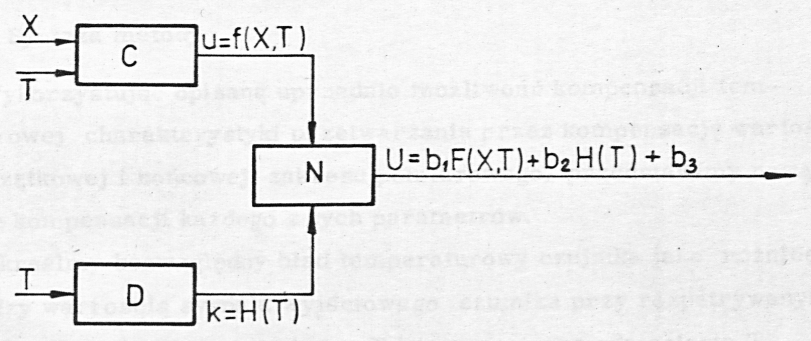
where: $b_{1}$ , $b_{2}$ , $b_{3}$ are independent of temperature (their temperature drift is included in the equivalent temperature error of the sensor) and of the measured value.

Differentiating and transforming (3) we obtain expressions for the lower range value $U_{p}$ and the sensitivity $\alpha_{1}$ :

\left\{ \begin{aligned} U_{p} &= U - X \frac{\partial U}{\partial X} \\ \alpha_{1} &= \frac{\partial U}{\partial X} \end{aligned} \right. \qquad (13)

Substituting expression (12) into (13) one obtains the equations:

\left\{ \begin{aligned} U_{p} &= b_{1} \left[ f(X, T) - X \frac{\partial f(X, T)}{\partial X} \right] + b_{2} \cdot H(T) + b_{3} \\ \alpha_{1} &= b_{1} \frac{\partial f(X, T)}{\partial X} \end{aligned} \right. \qquad (14)

which make the lower range value $U_{p}$ and the sensitivity $\alpha_{1}$ dependent on the functions f(X, T) and H(T). In order to determine the restrictions on these functions, and in connection with the adoption of the linear model of the transfer characteristic

s. 43

determined by relation (3), we shall check for (14) the conditions of temperature compensation (7). These conditions lead to two second-order partial differential equations:

\left\{ \begin{aligned} \frac{\partial H(T)}{\partial T} &= \frac{b_{1}}{b_{2}} \cdot \left[ X \cdot \frac{\partial^{2} f(X, T)}{\partial X \, \partial T} - \frac{\partial f(X, T)}{\partial T} \right] \\ \frac{\partial^{2} f(X, T)}{\partial X \cdot \partial T} &= 0 \end{aligned} \right. \qquad (15)

after solving which we have the sought conditions for the functions $H(T)$ and $f(X, T)$ :

H(T) = \frac{b_{1}}{b_{2}} \cdot \left[ X \cdot \frac{\partial f(X, T)}{\partial X} - f(X, T) \right] + f_{1}(X) + C_{1} \qquad (16)

f(X, T) = f_{2}(X) + f_{3}(T) + C_{2} \qquad (17)

where $f_{1}$ , $f_{2}$ , $f_{3}$ - arbitrary functions of one variable $C_{1}$ , $C_{2}$ - arbitrary constants

Thus the function $H(T)$ must have a course opposite to the temperature error of the sensor, determined by the first term of relation (16), and may be augmented by an arbitrary function of the measurand $f_{1}(X)$ and also by an arbitrary constant $C_{1}$ . The function $f(X, T)$ , on the other hand, may only be a sum of independent functions of pressure $f_{2}(X)$ and of temperature $f_{3}(T)$ , augmented by an arbitrary constant.

Relation (17) therefore expresses the condition of additivity of the value of the measured parameter and of the temperature error, formulated in Section 4.1 (c).

s. 44

4.3. The essence of complete temperature compensation

4.3.1. Synthesis of the method

Making use of the possibility, described above, of temperature compensation of the transfer characteristic by compensation of the lower and upper range values of the measuring range, we shall present a new method of compensation of each of these parameters.

Let us define the absolute temperature error of the sensor as the difference between the value of the sensor output signal at the pressure $X$ under consideration at a given temperature $T$ and at the reference temperature $T_{o}$ , denoting it by $\delta(T)$ :

\delta(T) = f(X, T) - f(X, T_{o}) \qquad (18)

Let us denote the maximum absolute value of the error 18 by $\delta_{m}$ ³

\delta_{m} = \left| \delta(T) \right|_{\max} \qquad (19)

In an analogous way we shall define the absolute temperature error of the transducer $\Delta(T)$

\Delta(T) = g(X, T) - g(X, T_{o}) \qquad (20)

and the maximum absolute value of the error (20) by $\Delta_{m}$

\Delta_{m} = \left| \Delta(T) \right|_{\max} \qquad (21)

If we denote by $U_{p}$ and $U_{k}$ respectively the values of the sensor output signal corresponding to the lower and upper range values of the measured pressure $X$ , then the effect of the action of the compensation circuit will be a reduction of the maximum relative measurement error of the transducer in comparison with the maximum relative error of the sensor (Fig. 16):

\frac{\delta_{m}}{\left| U_{k} - U_{p} \right|} > \frac{\Delta_{m}}{\left| U_{k} - U_{p} \right|} \qquad (22)

s. 45

Fig. 16. Illustration of the action of the compensation circuit

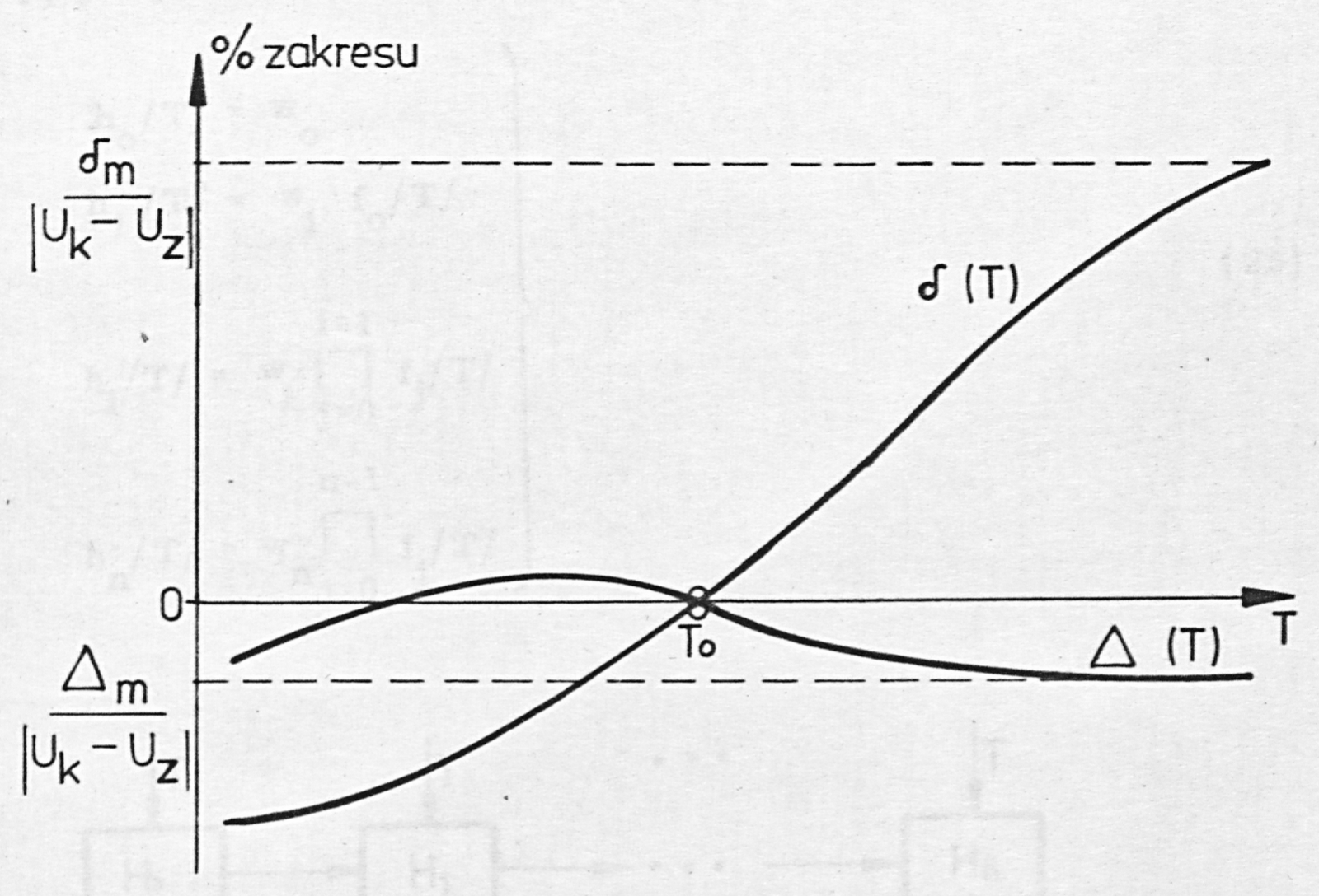
Labels: % zakresu = % of the measuring range⁴

Substituting expression (12) into relation (20), taking (18) into account, we obtain the definition of the temperature error of the transducer in the form

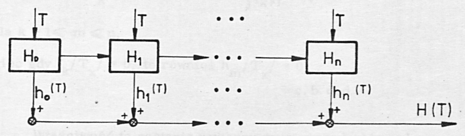
\Delta(T) = b_{1} \cdot \delta(T) + b_{2} \cdot H(T) \qquad (23)

Let the compensation circuit D (Fig. 15) be built of (n+1) generators $H_{o}$ , $H_{1}$ , ....., $H_{n}$ (Fig. 17). Each of the generators produces the compensating signals $h_{o}(T)$ ,..., $h_{n}(T)$ respectively. The output signal H(T) of the compensation circuit constitutes the sum of these signals:

H(T) = \sum_{i=0}^{n} h_{i}(T) \qquad (24)

Let us assume that the compensating signals $h_{o}(T)$ ,..., $h_{n}(T)$ are mutually related by means of the component functions⁵

s. 46

$f_{o}(T)$ ,...., $f_{n}(T)$ , dependent on temperature, in the following way⁶

\left. \begin{aligned} h_{o}(T) &= w_{o} \\ h_{1}(T) &= w_{1} \cdot f_{o}(T) \\ h_{i}(T) &= w_{i} \cdot \prod_{j=0}^{i-1} f_{j}(T) \\ h_{n}(T) &= w_{n} \cdot \prod_{j=0}^{n-1} f_{j}(T) \end{aligned} \right\} \qquad (25)

Fig. 17. Block diagram of the compensation circuit

where: $w_{o}$ , $w_{1}$ ,... $w_{n}$ - constants $i$ , $j$ , $n$ - natural numbers

Taking (25) and (24) into account, the expression describing the temperature error of the transducer (23) takes the form

\Delta(T) = b_{1} \cdot \delta(T) + b_{2} \cdot w_{o} + b_{2} \cdot \sum_{i=1}^{n} \left[ w_{i} \cdot \prod_{j=0}^{i-1} f_{j}(T) \right] \qquad (26)

Such a relationship between the compensating signals is characterised by the following property:

THEOREM 1

If at some temperature $T_{x}$ the value of the component function $f_{k}(T_{x})=0$ ,⁷

s. 47

where $k$ is a natural number $k < n$ , and the value of the constant $w_{k} \neq 0$ , then the compensating functions $h_{m}(T_{x}) = 0$ for natural $m$ in the interval $k + 1 \leqslant m \leqslant n$ , where $n$ is the number of component functions appearing in (25).

Proof: on the basis of (25) let us write

\frac{h_{m}(T_{x})}{h_{k}(T_{x})} = \frac{w_{m}}{w_{k}} \cdot f_{k}(T_{x}) \cdot \prod_{j=k+1}^{m} f_{j}(T_{x})

whence

h_{m}(T_{x}) = \frac{w_{m}}{w_{k}} \cdot f_{k}(T_{x}) \cdot h_{k}(T_{x}) \cdot \prod_{j=k+1}^{m} f_{j}(T_{x})

for $k + 1 \leqslant m \leqslant n$ ,

so that when $f_{k}(T_{x}) = 0$ , then also $h_{m}(T_{x}) = 0$

Q.E.D.

This property will be used to make the settings of the compensation circuit at different temperatures unidirectionally independent of one another. To this end let us make the component functions $f_{j}(T)$ dependent on the reference temperature $T_{o}$ and on the compensation temperatures $T_{1}$ ,..., $T_{n-1}$ as follows:

f_{j}(T) = a_{j}(T - T_{j}) \qquad (27)

where $a_{j}$ - constants $j = 0, 1, ..., n-1$

The adopted form (27) of the component functions $f_{j}(T)$ has the property of taking identically the value zero at the temperatures $T_{j}$

f_{j}(T_{j}) \equiv 0 \qquad (28)

s. 48

Taking (27) into account, the expression describing the temperature error of the transducer (26) takes the form

\Delta(T) = b_{1} \cdot \delta(T) + b_{2} w_{o} + b_{2} \cdot \sum_{i=1}^{n} w_{i} \cdot \prod_{j=0}^{i-1} \left[ a_{j}(T - T_{j}) \right] \qquad (29)

4.3.2. Compensation procedure

Let us now carry out the nulling of the temperature error of the transducer at the temperatures $T_{0}$ ,..., $T_{n}$ by changing the values of the coefficients $w_{i}$ , where for simplicity of the considerations we shall use relation (26) describing the temperature error of the transducer. We obtain in turn:⁸ $T = T_{o}$ ; the reference temperature

Using (28) we find

f_{o}(T_{o}) = 0

and taking (26) into account we obtain the value of the temperature error

\Delta(T_{o}) = b_{1} \cdot \delta(T_{o}) + b_{2} \cdot w_{o}

Since by assumption $\delta(T_{o}) = 0$ , the vanishing of the error $\Delta(T_{o})$ will occur for

w_{o} = 0 \qquad (30)

The coefficient $w_{o}$ could therefore be omitted from the further analysis. Since, however, at the reference temperature the standardization of the points of the transfer characteristic under consideration should be carried out, e.g. zero adjustment or setting the required value of the full-scale signal, in the further considerations the coefficient $w_{o}$ has been retained as a symbol of bringing the transfer error (and not the temperature error) to zero.

s. 49

$T = T_{1}$ : the first compensation temperature

At this temperature

f_{1}(T_{1}) = 0

as a result of which the temperature error (26), after taking into account the condition for $w_{o}$ obtained at $T=T_{o}$ , is determined:

\Delta(T_{1}) = b_{1} \cdot \delta(T_{1}) + b_{2} \cdot w_{1} \cdot f_{o}(T_{1})

The vanishing of the error $\Delta(T_{1})$ is obtained for the value $w_{1}$ :⁹

w_{1} = - \frac{b_{1} \; \delta(T_{1})}{b_{2} \; f_{o}(T_{1})} \qquad (31)

The required value of $w_{1}$ depends only on the ratio of the value of the sensor error $\delta(T)$ to the value of the component function $f_{o}(T)$ at this temperature, modified by the coefficients $b_{1}$ , $b_{2}$ of the normalizing circuit

$T = T_{2}$ : the second compensation temperature

Analogously to the above we obtain

f_{2}(T_{2}) = 0

and taking (26) into account we obtain the expression for the temperature error

\Delta(T_{2}) = b_{1} \cdot \delta(T_{2}) + b_{2} \cdot \left[ w_{o} + w_{1} \cdot f_{o}(T_{2}) + w_{2} \cdot f_{o}(T_{2}) \cdot f_{1}(T_{2}) \right]

whence, after equating to zero and substituting the conditions (30) and (31) for the constants $w_{o}$ and $w_{1}$ , one obtains the condition for the constant $w_{2}$ ¹⁰

w_{2} = - \frac{b_{1}}{b_{2}} \cdot \frac{\delta(T_{2}) - \frac{\delta(T_{1})}{f_{o}(T_{1})} \cdot f_{o}(T_{2})}{f_{o}(T_{2}) \cdot f_{1}(T_{2})} \qquad (32)

s. 50

Thus the value of the constant $w_{2}$ required to null the temperature error of the transducer at the temperature $T_{2}$ depends on the values of the sensor error at the first and second compensation temperatures ( $\delta(T_{1})$ and $\delta(T_{2})$ respectively) and on the values of the component functions $f_{o}(T)$ , $f_{1}(T)$ at both temperatures. It does not, however, depend on the values of the sensor error and the values of the component functions at the subsequent compensation temperatures.¹¹
At the same time it should be emphasised that fixing the value of the constant $w_{2}$ at the temperature $T_{2}$ does not affect the value of the constant $w_{1}$ , fixed at the first compensation temperature $T_{1}$ .

$T = T_{3}$ ..... $T_{k}$ .... $T_{n-1}$ : the subsequent compensation temperatures

Proceeding in a manner analogous to that presented above, one obtains at each of the compensation temperatures $T_{k}$ a condition for the constant $w_{k}$ (k = 3, 4,....., n-1) in the general form

w_{k} = - \frac{b_{1} \cdot \delta(T_{k}) + b_{2} \cdot w_{o} + b_{2} \cdot \sum_{i=1}^{k-1} w_{i} \cdot \prod_{j=0}^{i-1} f_{j}(T_{k})}{b_{2} \cdot \prod_{j=0}^{k-2} f_{j}(T_{k})} \qquad (33)

As before, the value of the constant $w_{k}$ necessary to obtain a zero value of the temperature error of the transducer at the temperature $T_{k}$ depends on the values of the constants $w_{o}$ ,... $w_{k-1}$ fixed at the previous temperatures and on the values of the component functions $f_{o}(T)$ ,......, $f_{k-1}(T)$ at the temperature $T_{k}$ , and on the values of the coefficients $b_{1}$ , $b_{2}$ of the normalizing circuit. The value of the constant $w_{k}$ does not, however, depend on the values of the constants $w_{k+1}$ ,....., $w_{n-1}$ and of the component functions $f_{k}(T)$ ,....., $f_{n-2}(T)$ at the subsequent compensation temperatures $T_{k+1}$ ,..... $T_{n-1}$ .

Making use of this property for the practical application of the method presented, we find that there exists a unidirectional independence of the settings of the elements fixing the values of the constants $w_{o}$ ,...., $w_{n-1}$ .

s. 51

$T = T_{n}$ : the last compensation temperature

At the previous temperatures the properties (28) of the vanishing of all the existing component functions $f_{j}(T)$ , (j=0, 1,..., n-1), have been exhausted in fixing the values of the constants $w_{i}$ , (i = 1, 2,...,n-1), necessary for compensating the error. Let us now choose the constant $w_{n}$ so as to obtain, for the last time, a zero value of the error $\Delta(T_{n})$

\Delta(T_{n}) = b_{1} \cdot \delta(T_{n}) + b_{2} \cdot w_{o} + b_{2} \cdot \sum_{i=1}^{n-1} w_{i} \cdot \prod_{j=0}^{i-1} f_{j}(T_{n}) + b_{2} \cdot w_{n} \cdot \prod_{j=0}^{n-2} f_{j}(T_{n})

whence

w_{n} = - \frac{b_{1} \cdot \delta(T_{n}) + b_{2} \cdot w_{o} + b_{2} \cdot \sum_{i=1}^{n-1} w_{i} \cdot \prod_{j=0}^{i-1} f_{j}(T_{n})}{b_{2} \cdot \prod_{j=0}^{n-2} f_{j}(T_{n})} \qquad (34)

Condition (34) has a form and properties analogous to expression (33), with the sole difference that there are no subsequent compensation temperatures. As a result of applying the method presented, one obtains a zero value of the temperature error of the point of the characteristic of the measuring transducer under consideration at n temperatures $T_{1}$ , $T_{2}$ ,......., $T_{n}$ , which means that at these temperatures the value of the point of the characteristic under consideration is equal to its value at the reference temperature $T_{o}$ .
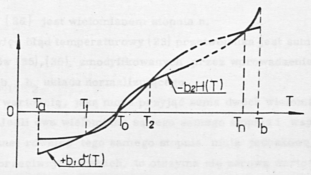
In the graphical interpretation of the action of the compensation method presented, the graph representing the dependence of the sensor-error component $b_{1}$ $\delta$ (T) in the transducer output signal will intersect the graph of the compensating-signal component $b_{2}$ $H(T)$ with reversed sign at (n+1) temperature points (Fig. 18).¹²

s. 52

Fig. 18. Graphical interpretation of the action of n-point compensation

4.3.3. Sufficient conditions for complete temperature compensation

The condition of zero temperature error of the transducer at n compensation temperatures is not sufficient to determine its maximum value. For this, knowledge of the value of the error over the whole operating temperature range under consideration is necessary. We shall now consider the sufficient conditions for complete temperature compensation in the sense of minimization of the value of the temperature error.
Let us introduce the following description of the temperature error of the sensor $\delta(T)$

\delta(T) = c_{o} + c_{1} T + c ... + c_{s} \; T^{s} \qquad (35)

where $c_{o}$ ,..., $c_{s}$ - constants

By virtue of the Weierstrass approximation theorem [83] (see Section 4.2), expression (35) approximates any continuous curve sufficiently accurately, the degree s of the approximating polynomial being a function of the accuracy of approximation. Let us therefore assume that the description (35) of the temperature error of the sensor is a sufficiently accurate representation of the real error (18) of the sensor. Comparing expressions (29) and (23) we may determine the compensating signal as follows

s. 53

H(T) = w_{o} + \sum_{i=1}^{n} w_{i} \cdot \prod_{j=0}^{i-1} a_{j} \cdot (T - T_{j}) \qquad (36)

Expression (36) is a polynomial of degree n. Thus the temperature error (23) of the transducer is the sum of two polynomials (35), (36), modified by the introduction of the coefficients $b_{1}$ , $b_{2}$ of the normalizing circuit. The minimum value that the sum of two polynomials can take is zero. If two polynomials are of the same degree and the coefficients of the variable of the same degree likewise have equal absolute values and opposite signs, then a zero value of the sum of these polynomials is obtained irrespective of the value of the variable. We may therefore formulate the conclusion that the optimum condition of temperature compensation that interests us is the attainment of the identity

b_{1} \cdot \delta(T) + b_{2} \cdot H(T) \equiv 0 \qquad (37)

A necessary condition for attaining (37) is the equality of the degrees of the polynomials (35) and (36):

n = s \qquad (38)

which is equivalent to equating the number n of compensation temperatures with the degree s of the polynomial approximating the temperature error of the sensor. As a result of carrying out the compensation in accordance with Section 4.3.2, one obtains (n+1) zeros of the equation:

\Delta(T) = 0

Since through (n+1) points only one curve of degree n can be drawn, this means that the compensation procedure leads unambiguously to the identity (37). This is equivalent to the identical vanishing of the temperature error of the transducer over the whole operating temperature range, irrespective of the choice of the compensation temperatures.
In the analysis carried out above it was assumed that the compensating-signal generators $H_{1}$ ... $H_{n}$ produce signals linearly dependent on temperature. The resultant compensating signal is produced

s. 54

by establishing an appropriate combination of products of these signals, giving as a result a polynomial of degree $n$ . Let us now assume that we wish to obtain a polynomial of degree $n$ with a smaller number of compensation temperatures. To this end let us make the component functions $f_{j}(T)$ dependent on temperature in the following way:

f_{j}(T) = (T - T_{j}) \cdot \sum_{p=0}^{m-1} a_{jp} \cdot (T - T_{j})^{p} \qquad (39)

where $a_{jp}$ - constants $j = 0, 1, ..., n-1$
$m$ - a natural number

Expression (39) is a polynomial of degree $m$ and, by virtue of the Weierstrass approximation theorem [83] (see Section 4.2), it can describe any continuous function, the degree $m$ of the polynomial depending on the required accuracy of approximation of that function. The adopted form (39) of the component functions $f_{j}(T)$ also has the property (28) of vanishing identically at the temperatures $T_{j}$ .
Let us assume in turn that a certain number $R$ of properties of relation (35) approximating the temperature error of the sensor is known in advance. Let the degree $m$ of the component function (39) be determined as follows

m = R + r \qquad (40)

where $r$ is a natural number

By raising the degree $m$ one obtains a compensating polynomial $H(T)$ of degree $n(R+r)$ . In order to obtain the identity (37) the relation

s = n(R + r) \qquad (41)

must be satisfied, whence one obtains the required number $n$ of compensation temperatures in the case of adopting $r = 0$ , that is, in the case of maximum use of the $R$ known properties:

n = \frac{s}{R} \qquad (42)

s. 55

Conclusions: the optimum conditions of complete temperature compensation can be achieved either by producing component functions $f_j(T)$ linear as a function of temperature and carrying out the compensation at a number of temperatures equal to the degree of the polynomial describing the temperature error of the sensor (condition 38), or else by raising the degree of the polynomial describing the component function $f_j(T)$ , relying on properties of the temperature error of the sensor known in advance, and reducing the number of compensation temperatures (condition 42).

An example of advance information on the character of the temperature error of the sensor is information on the ratio of the values of the errors at certain temperatures. Thus in integrated pressure sensors [40] the temperature span drift is approximated by a fourth-order curve, and the quotient of the values of the temperature error at the temperatures 352 K and 241 K is a function of the substrate resistivity. In such a case it may prove sufficient to produce a function $f_j(T)$ compensating the temperature error of one sensor, which will then make it possible to compensate all the sensors by multiplying (dividing) the value of the compensating signal by an appropriate proportionality coefficient.

s. 56

The method will now be explained by examples.

Example 1

Let the sensor error be determined by the quadratic relation

\delta(T) = B \cdot (T - T_{o}) \cdot (T + T_{x})

where $T_{x}$ - a constant and let $b_{1} = b_{2} = 1$

We shall realise two variants of the compensation circuit for $m \cdot n = 2$ ; subjecting them next to compensation, we shall carry out the compensation procedures for them

variant (a) $n = 2$ $m = 1$ , so

f_{o} = a_{1} \cdot (T - T_{o})

f_{1} = a_{2} \cdot (T - T_{1})

and after substitution into (26) we obtain

\Delta(T) = B \cdot (T - T_{o}) \cdot (T + T_{x}) + w_{o} + w_{1} \cdot a_{1} \cdot (T - T_{o}) - w_{2} \cdot a_{1} \cdot a_{2} \cdot (T - T_{o}) \cdot (T - T_{1})

Compensation procedure:

T = T_{o}; \quad \Delta(T_{o}) = w_{o}

and hence we obtain the condition for the vanishing of the error $\Delta(T_{o})$ ¹³ ¹⁴

w_{o} = 0

T = T_{1}; \quad \Delta(T_{1}) = B \cdot (T_{1} - T_{o}) \cdot (T_{1} + T_{x}) + w_{1} \cdot a_{1} \cdot (T - T_{o})

and the condition for the vanishing of the error $\Delta(T_{1})$ ¹⁵

w_{1} = - \frac{B \cdot (T_{1} + T_{x})}{a_{1}}

T = T_{2};

\Delta(T_{2}) = B \cdot (T_{2} - T_{o}) \cdot (T_{2} + T_{x}) + B \cdot (T_{1} + T_{x}) \cdot (T_{2} - T_{o}) - a_{1} \cdot a_{2} \cdot w_{2} \cdot (T_{2} - T_{o}) \cdot (T_{2} - T_{1})

s. 57

and finally the condition for the vanishing of the error $\Delta(T_{2})$

w_{2} = - \frac{B}{a_{1} \cdot a_{2}}

Substituting the values $w_{o}$ , $w_{1}$ , $w_{2}$ obtained in this way into expression (26), one obtains the identity

\Delta(T) \equiv 0

variant (b) $n = 1$ , $m = 2$

f_{o}(T) = (T - T_{o}) \cdot (a_{o1} + a_{o2} T)

After substitution into (26) we obtain

\Delta(T) = B \cdot (T - T_{o}) \cdot (T + T_{x}) + w_{o} + w_{1} \cdot (T - T_{o}) \cdot (a_{o1} + a_{o2} \cdot T)

Compensation procedure¹⁶

T = T_{o}; \quad \Delta(T_{o}) = w_{o} \qquad \text{whence}

w_{o} = 0

T = T_{1}; \quad \Delta(T_{1}) = B \cdot (T_{1} - T_{o}) \cdot (T_{1} + T_{x}) + w_{1} \cdot (T_{1} - T_{o}) \cdot (a_{o1} + a_{o2} \cdot T_{1})

whence¹⁷

w_{1} = - \frac{B \cdot (T_{1} + T_{x})}{a_{o1} + a_{o2} \cdot T_{1}}

Taking into account the values of $w_{o}$ and $w_{1}$ obtained, we obtain

\Delta(T) = B \cdot (T - T_{o}) \cdot \left[ T + T_{x} - \frac{(T_{1} + T_{x}) \cdot (T + \frac{a_{o1}}{a_{o2}})}{T_{1} + \frac{a_{o1}}{a_{o2}}} \right]

The value of $\Delta(T)$ obtained is identically equal to zero under the additional

s. 58

condition, relating its sensor-error characteristic to the characteristic of the compensating signal, in the form

T_{x} = \frac{a_{o1}}{a_{o2}}

This is obvious, since complete compensation of an error described by a quadratic function requires three degrees of freedom (balancing of the three coefficients $T_{o}$ , $T_{x}$ , B), whereas in the compensation procedure of variant b we have only two degrees of freedom, namely the coefficients $w_{o}$ and $w_{1}$ . The procedure presented according to variant a is based on three degrees of freedom - the coefficients $w_{o}$ , $w_{1}$ and $w_{2}$ - and consequently no additional condition was required.

4.4. The essence of incomplete temperature compensation

We shall now consider the value of the error (26) of the transducer under the assumption of incomplete compensation. By incomplete compensation will be understood a limitation of the number of compensation temperatures in comparison with the values obtained from relations (38) or (42).

m \cdot n < s \qquad (43)

For simplicity this compensation will be shown for the case of the degree s of the polynomial approximating the temperature error of the sensor equal to two and three, which practically exhausts almost all the cases met with in practice. In the case $s = 1$ the temperature error is reduced identically to zero by a compensation circuit with the parameters $m = 1$ , $n = 1$ .

4.4.1. Case: $s = 2$ , $m = 1$ , $n = 1$

In this case the sensor error is described by the relation

\delta(T) = B \cdot (T - T_{o}) \cdot (T + T_{x}) \qquad (44)

where $T_{o}$ - the reference temperature B, $T_{x}$ - constants

s. 59

On the basis of (27) we have $f_{o} = a_{o} \cdot (T - T_{o})$ and using (26) we shall write the error $\Delta(T)$ of the transducer in the form

\Delta(T) = b_{1} \cdot B \cdot T^{2} + \left[ b_{1} \cdot B \cdot (T_{x} - T_{o}) + b_{2} \cdot w_{1} \cdot a_{o} \right] \cdot T - b_{1} \cdot B \cdot T_{o} \cdot T_{x} - b_{2} \cdot w_{1} \cdot a_{o} \cdot T_{o}

The compensation procedure is as follows:

a. $T = T_{o}$ ; $\Delta(T_{o}) = 0$

b. $T = T_{1}$ ;

\Delta(T_{1}) = b_{1} \cdot B \cdot \left[ T_{1}^{2} + (T_{x} - T_{o}) \cdot T_{1} - T_{o} \cdot T_{x} \right] - w_{1} \cdot b_{2} \cdot a_{o} \cdot (T_{o} - T_{1})

In order to bring the error $\Delta(T_{1})$ to zero the value $w_{1}$ is necessary:

w_{1} = \frac{b_{1} \cdot B \cdot \left[ T_{1}^{2} + (T_{x} - T_{o}) \cdot T_{1} - T_{o} \cdot T_{x} \right]}{b_{2} \cdot a_{o} \cdot (T_{o} - T_{1})} \qquad (45)

Introducing the value $w_{1}$ obtained into (45), we obtain the relation describing the temperature error of the compensated transducer¹⁸

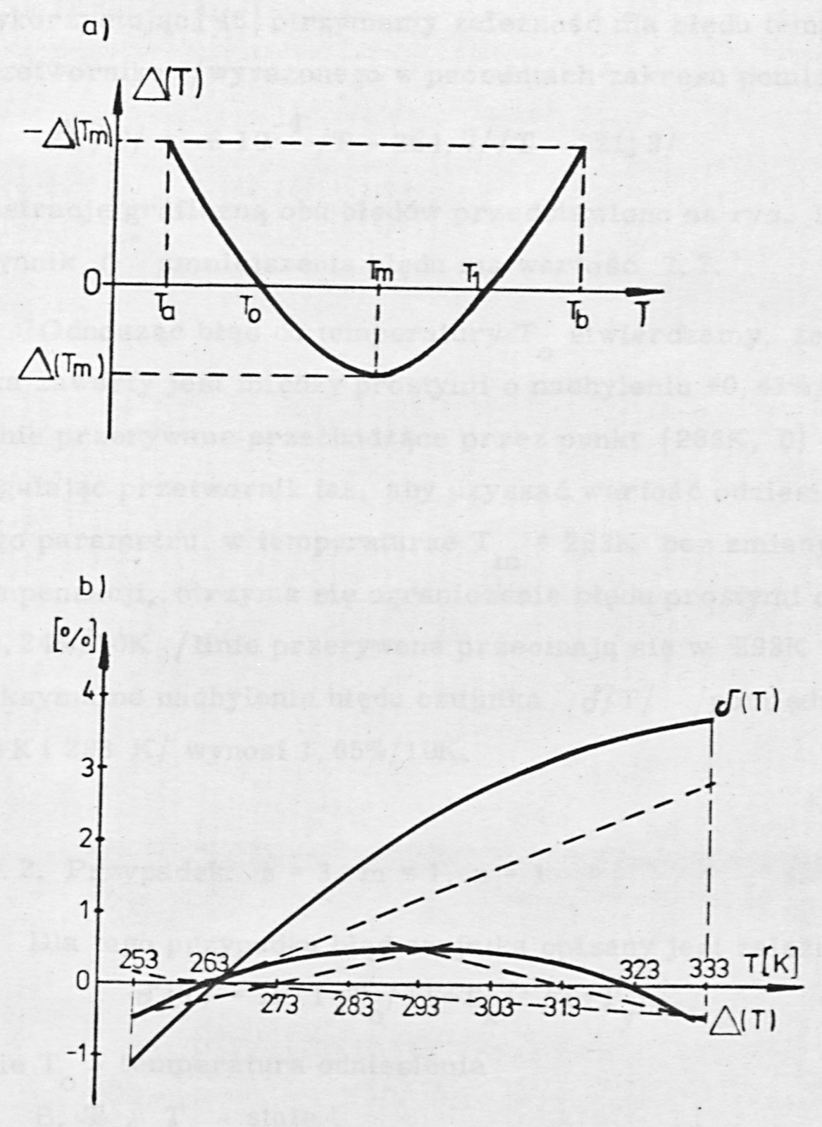
\Delta(T) = b_{1} \cdot B \cdot (T - T_{o}) \cdot (T - T_{1}) \qquad (46)

Let us impose an additional condition, requiring that the values of the error (73) at the limits $T_{a}$ , $T_{b}$ of the operating temperature range be equal to each other and that they be equal - with opposite sign - to the value of the error at the temperature $T_{m}$ at which the extremum of the function occurs (Fig. 19a):¹⁹

\Delta(T_{a}) = \Delta(T_{b}) = -\Delta(T_{m}) \qquad (47)

it can therefore easily be shown that

T_{m} = \frac{T_{o} + T_{1}}{2} \qquad (48)

and

\Delta(T_{m}) = - \frac{b_{1} \cdot B \cdot (T_{o} - T_{1})^{2}}{4} \qquad (49)

Assuming $T_{a} < T_{b}$ , $T_{o} < T_{1}$ , the value of the reference temperature $T_{o}$ will be determined by the relation

s. 60

T_{o} = T_{a} + \frac{\sqrt{2} - 1}{2\sqrt{2}} \cdot (T_{b} - T_{a}) \qquad (50)

while the first compensation temperature $T_{1}$ :

T_{1} = T_{b} - \frac{\sqrt{2} - 1}{2\sqrt{2}} \cdot (T_{b} - T_{a}) \qquad (51)

The error-reduction factor $\eta$ of the temperature error of the sensor will be determined as follows:

\eta = \left| \frac{\delta m}{\Delta m} \right| = \left| \frac{T_{b} + T_{x}}{b_{1} \cdot (T_{b} - T_{1})} \right| \qquad (52)

As can be seen, condition (47) unambiguously makes the values of the reference temperature and of the first compensation temperature dependent on the limit temperatures of operation, irrespective of the parameters of the sensor and of the compensation circuit (which should merely lead to condition 47).

The value of the maximum temperature error of the transducer is also in such a case independent of the parameters of the compensation circuit. For, substituting (50) and (51) into (49), we obtain the value of the extreme error of the transducer $\Delta(T_{m})$ :

\Delta(T_{m}) = - \frac{b_{1} \cdot B}{8} \cdot (T_{b} - T_{a})^{2} \qquad (53)

and so this value depends only on the width of the operating temperature range and on the uncompensated constant B of the sensor-error characteristic, and on the constant $b_{1}$ of the normalizing circuit.

Example 2

The transducer is to operate in the temperature range 253 K to 333 K. On the basis of (51) and (52) we calculate: $T_{o}$ = 264.7 K, $T_{1}$ = 321.3 K. The sensor error referred to the temperature $T_{o}$ we shall describe by the relation (expressed²⁰

s. 61

Fig. 19. Temperature error of the sensor δ(T) and of the transducer Δ(T) in the case s = 2

s. 62

as a percentage of the measuring range):²¹

\Delta(T) = - 6\ 10^{-4} \cdot (T - 264.7) \cdot (T - 423)

and for simplicity we shall adopt the parameters of the normalizing circuit $b_{1} = b_{2} = 1$ . Using (46) we obtain the relation for the temperature error of the transducer (expressed as a percentage of the measuring range):

\Delta(T) = -6\ 10^{-4} \cdot (T - 264.7) \cdot (T - 321.3)

A graphical illustration of both errors is presented in Fig. 19b. The error-reduction factor $\eta$ has the value 7.7.

Referring the error to the temperature $T_{o}$ , we find that the transducer error is contained between straight lines of slope +0.41 %/10 K and 0.07 %/10 K (dashed lines passing through the point (283 K, 0) in Fig. 19b). Adjusting the transducer so as to obtain the reference value of the parameter under consideration at the temperature $T_{m}$ = 293 K without changing the compensation parameters, one obtains a limitation of the error by straight lines of slope ± 0.24 %/10 K (dashed lines intersecting at 293 K in Fig. 19b). The maximum slope of the sensor error $\delta(T)$ (between the temperatures 253 K and 293 K) amounts to 1.05 %/10 K.

4.4.2. Case: $s = 3$ , $m = 1$ , $n = 1$

For this case the sensor error is described by the relation:

\delta(T) = B \cdot (T - T_{o}) \cdot (T + T_{x}) \cdot (T + T_{y}) \qquad (54)

where $T_{o}$ - the reference temperature B, $T_{x}$ , $T_{y}$ - constants

On the basis of (27) we therefore write

f_{o} = a_{o} \cdot (T - T_{o})

and taking $w_{o} = 0$ into account we obtain the transducer error in the form

\Delta(T) = b_{1} \cdot B \cdot (T - T_{o}) \cdot (T + T_{x}) \cdot (T + T_{y}) + b_{2} \cdot w_{1} \cdot a_{o} \cdot (T - T_{o})

s. 63

The temperature compensation procedure is as follows:²²

T = T_{o}; \quad \Delta(T_{o}) = 0

T = T_{1}; \quad \Delta(T_{1}) = b_{1} \cdot B \cdot (T_{1} - T_{o}) \cdot (T_{1} + T_{y}) + b_{2} \cdot w_{1} \cdot a_{o} \cdot (T_{1} - T_{o})

In order to bring $\Delta(T_{1})$ to zero the value $w_{1}$ is required

w_{1} = - \frac{b_{1} \cdot B \cdot (T_{1} + T_{x}) \cdot (T_{1} + T_{y})}{b_{2} \cdot a_{o}} \qquad (55)

Taking into account the value (55) obtained for $w_{1}$ , one obtains the relation for the error of the compensated transducer

\Delta(T) = b_{1} \cdot B \cdot (T - T_{o}) \cdot \left[ T^{2} + (T_{x} + T_{y}) \cdot T - T_{1}^{2} \cdot (T_{x} + T_{y}) \right] \qquad (56)

It may be assumed that, from the point of view of the needs of compensation, it will be advantageous for relation (56) to be characterised by the following features: (a) that it should have 3 real roots; this will be satisfied when the discriminant D of the quadratic equation in square brackets in relation (56)

\Delta = (T_{x} + T_{y} + 2T_{1})^{2}

is greater than zero, that is, for every $T_{1}$ satisfying the condition:

T_{1} \neq - \frac{T_{x} + T_{y}}{2}

(b) that both roots of the equation in square brackets in relation (56) should lie within the operating temperature range: this condition cannot, however, be guaranteed with a single degree of freedom in the form of the constant $T_{1}$ .

The minimization of the error (56) for assumed spreads of the parameters $T_{x}$ and $T_{y}$ can be carried out most quickly by means of computer calculations of variants on the basis of the results of measurement of the sensor error.

Example 3

Operating temperature range from 253 K to 333 K. Sensor error

s. 64

Fig. 20. Temperature error of the sensor δ(T) and of the transducer Δ(T) in the case s = 3, m = 1, n = 1.

s. 65

\delta(T) = -1.8 \cdot 10^{-5} \cdot (T - 263)(T - 238.3) \cdot (T - 382.7)

Constants $b_{1} = b_{2} = 1$

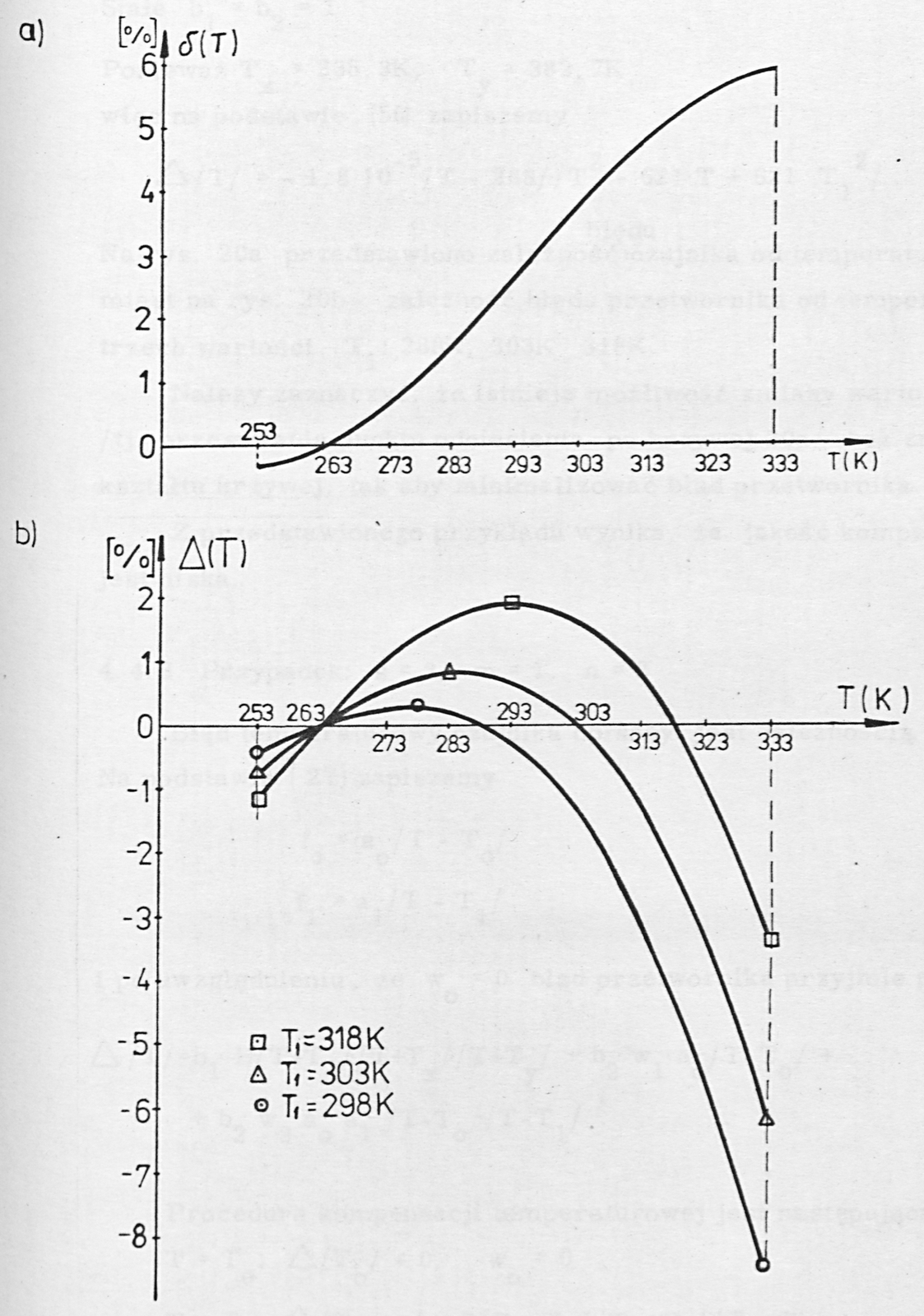
Since $T_{x}$ = 238.3 K, $T_{y}$ = 382.7 K on the basis of (56) we therefore write

\Delta(T) = - 1.8 \cdot 10^{-5} \cdot (T - 263) \cdot (T^{2} - 621 \cdot T + 621 \cdot T_{1}^{2})

Fig. 20a presents the dependence of the sensor error on temperature, while Fig. 20b presents the dependence of the transducer error on temperature for three values of $T_{1}$ : 288 K, 303 K, 318 K.²³

It should be noted that there is the possibility of changing the value of $T_{o}$ (i.e. shifting the reference point along the curve 20a) without changing the shape of the curve, so as to minimize the transducer error.

From the example presented it follows that the quality of the compensation is low.

4.4.3. Case: s = 3, m = 1, n = 2

The temperature error of the sensor is described by relation (54). On the basis of (27) we write

f_{o} = a_{o} \cdot (T - T_{o})

f_{1} = a_{1} \cdot (T - T_{1})

and taking into account that $w_{o} = 0$ , the transducer error takes the form

\Delta(T) = b_{1} \cdot B (T - T_{o}) \cdot (T + T_{x}) \cdot (T + T_{y}) + b_{2} \cdot w_{1} \cdot a_{o} \cdot (T - T_{o}) +

+ b_{2} \cdot w_{2} \cdot a_{o} \cdot a_{1} (T - T_{o}) \cdot (T - T_{1})

The temperature compensation procedure is as follows:

T = T_{o}; \quad \Delta(T_{o}) = 0, \qquad w_{o} = 0

T = T_{1}; \quad \Delta(T_{1}) = b_{1} \cdot B (T_{1} - T_{o}) \cdot (T_{1} + T_{x}) \cdot (T_{1} + T_{y}) + b_{2} \cdot w_{1} \cdot a_{o} \cdot (T_{1} - T_{o}) +

+ b_{2} \cdot w_{2} \cdot a_{o} \cdot a_{1} \cdot (T_{1} - T_{o})

s. 66

The value $w_{1}$ bringing the error $\Delta(T_{1})$ to zero we shall write

w_{1} = - \frac{b_{1} \cdot B (T_{1} + T_{x}) \cdot (T_{1} + T_{y})}{b_{2} \cdot a_{o}} \qquad (57)

Taking into account the value of $w_{1}$ found, the expression for the transducer error takes the form

\Delta(T) = b_{1} \cdot B (T - T_{o}) \cdot (T + T_{x}) \cdot (T + T_{y}) - b_{1} \cdot B (T_{1} + T_{x}) \cdot (T_{1} + T_{y}) \cdot (T - T_{o}) +

+ b_{2} \cdot w_{2} \cdot a_{o} \cdot a_{1} \cdot (T - T_{o}) \cdot (T - T_{1})

$T = T_{2}$ ; determining the error analogously to the above, we obtain the value $w_{2}$ nulling it:

w_{2} = - \frac{b_{1} \cdot B (T_{2} + T_{x}) \cdot (T_{2} + T_{y}) - b_{1} \cdot B (T_{1} + T_{x}) \cdot (T_{1} + T_{y})}{b_{2} \cdot a_{o} \cdot a_{1} \cdot (T_{2} - T_{1})} \qquad (58)

After substituting the values of $w_{1}$ and $w_{2}$ found, we obtain the relation describing the temperature error of the compensated transducer:²⁴

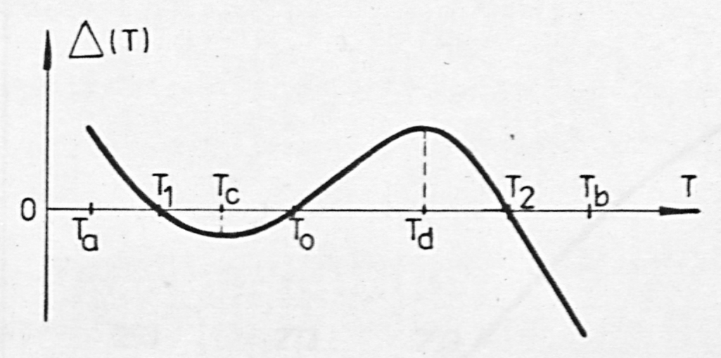
\Delta(T) = b_{1} \cdot B (T - T_{o}) \cdot (T - T_{1}) \cdot (T - T_{2}) \qquad (59)

This error depends on the value of the uncompensated constant B of the sensor error, on the values of the compensation temperatures $T_{1}$ and $T_{2}$ and of the reference temperature $T_{o}$ , and is at the same time modified by the coefficient $b_{1}$ of the normalizing circuit. Relation (59) guarantees obtaining three zeros within the operating temperature range (Fig. 21). Imposing the condition of values of the error $\Delta(T)$ equal in absolute value at the extrema occurring at the temperatures $T_{c}$ , $T_{d}$ , one obtains a relation between the reference temperature and the compensation temperatures:

T_{o} = \frac{T_{1} + T_{2}}{2} \qquad (60)

The value of the maximum error can be shaped by changing the differences between the compensation temperatures and by changing the value of the reference temperature.

s. 67

Fig. 21. Desired course of the transducer error in the case s = 3, m = 1, n = 2

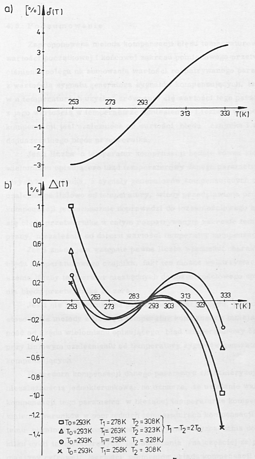
Example 4

Operating temperature range from 253 K to 333 K The sensor error is described by the curve (Fig. 22)

\delta(T) = - 1.8 \cdot 10^{-5} \cdot (T - 293) \cdot (T - 373) \cdot (T - 218)

constants $b_{1} = b_{2} = 1$

Thus, $T_{x} = - 373K$ , $T_{y} = - 218K$ , $B = - 1.8 \cdot 10^{-5}$

The dependence of the error (59) of the compensated transducer on temperature depends on the choice of the compensation temperatures $T_{1}$ and $T_{2}$ :²⁵

\Delta(T) = - 1.8 \cdot 10^{-5} \cdot (T - 293)(T + T_{1}) \cdot (T + T_{2})

Graphs of this error for various pairs $T_{1}$ , $T_{2}$ satisfying (60), and for one pair not satisfying (60), are presented in Fig. 22b.

s. 68

Fig. 22. Temperature error of the sensor: δ(T) and of the transducer Δ(T) in the case s = 3, m = 1, n = 2

²⁶

s. 69

4.5. Summary

The proposed method of compensation of the temperature error of the lower and upper range values of the measuring range of a pressure transducer consists in summing the value of the parameter under consideration with the value of the signal of the compensating-signal generator, so that at n temperatures the value of this parameter becomes equal to its value at the reference temperature. The number n of compensation temperatures depends on the value of the sensor error and on the value of the permissible transducer error.

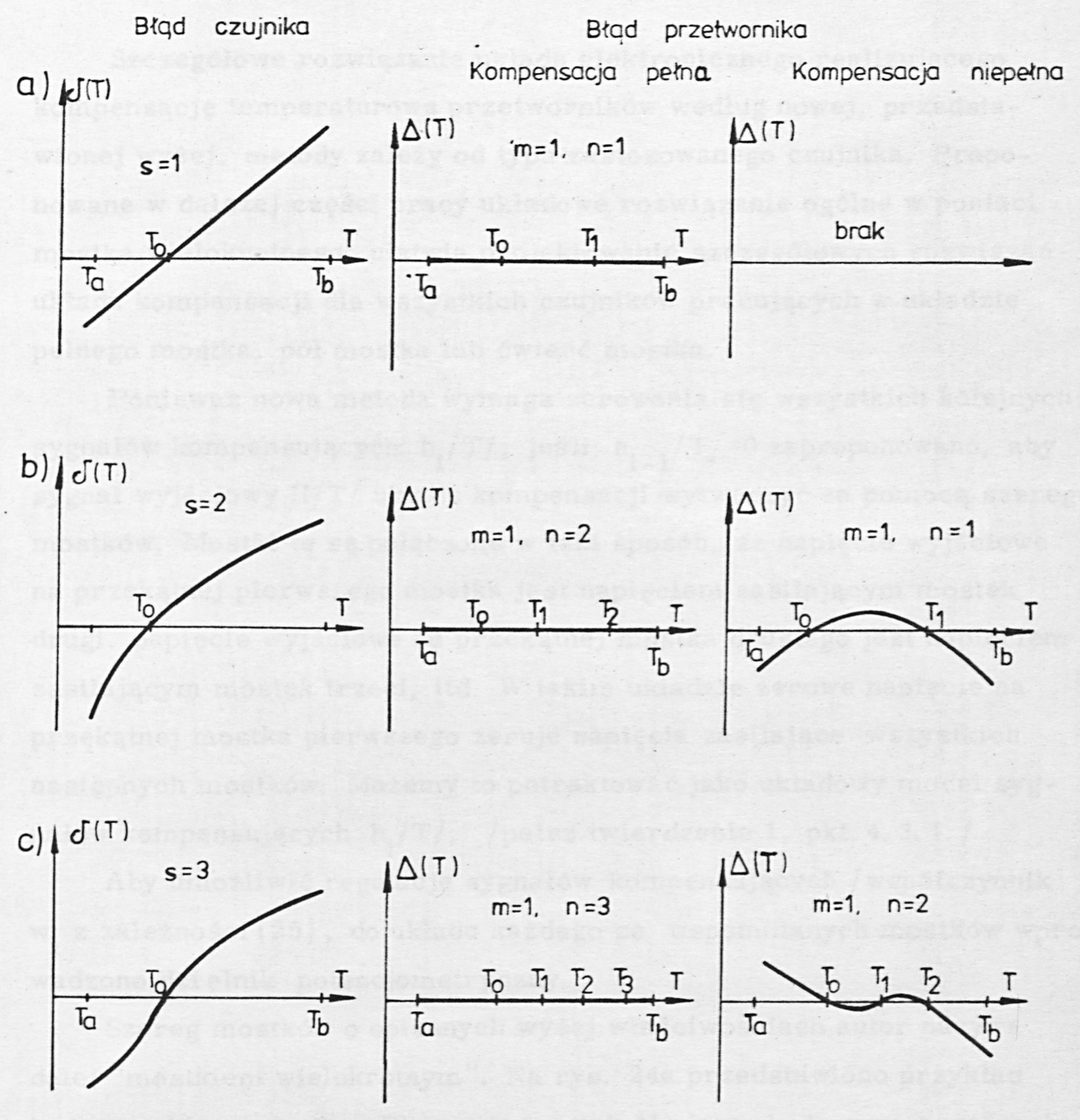
If the number n of compensation temperatures is equal to the degree of the polynomial describing the temperature error of the given parameter of the sensor characteristic, and the signals of the compensating generators are linearly dependent on temperature, then the compensation procedure presented leads unambiguously to the identical vanishing of the transducer error over the whole operating temperature range under consideration, irrespective of the choice of the values of the compensation temperatures.

If a certain number of properties of the temperature-error characteristic of the sensor is known in advance, this fact can be used to reduce the number of temperatures necessary for reducing the transducer error identically to zero.

If complete compensation of the error is not required, it is proposed to use the method with a number n of compensation temperatures smaller by one than the degree of the polynomial describing the temperature error of the sensor, with the signals of the compensating generators linearly dependent on temperature.

The compensation procedure for a given parameter is characterised by unidirectional independence, which means that establishing the compensation conditions for this parameter at the current compensation temperature does not change the conditions at the previous compensation temperatures. Thanks to this, the necessity is eliminated of iterative determination, which requires several temperature cycles, or of calculation (most often by means of a digital computer) of the values of the components of the compensation circuit necessary for compensating the temperature error of the parameter of the transducer characteristic

s. 70

under consideration.

Comparing the method presented with other known methods [1, 32–76], it must be stated that only the method presented in this thesis makes possible the identical reduction of the temperature error of the transducer to zero together with unidirectional independence of the establishment of the compensation conditions.

In the method presented, the change of the temperature characteristic of the compensating signal is effected by changing proportionality coefficients that are independent of temperature. In practical application the compensation method may consist in appropriately setting potentiometric dividers of the compensating signals. Since on such dividers only a signal of the order of the temperature errors of the sensor would then be present, that is, a small percentage of the full-scale signal, the metrological requirements imposed on these components could be relaxed.

The use of the potentiometric dividers mentioned would eliminate the necessity of stocking a large number of values of compensating components (which may potentially be used) or of manufacturing them after obtaining information on the sensor errors.

The method presented can be applied in measuring transducers of all types for non-electrical quantities satisfying the conditions listed in Section 4.1.

Fig. 23 presents schematically the course of the temperature error of a compensated transducer in the case of complete compensation and of incomplete compensation for the cases most frequently met with in practice.

s. 71

Fig. 23. Schematic shape of the temperature error Δ(T) of a compensated transducer in the case of complete and incomplete compensation; a. sensor error δ(T) described by a linear function; b. sensor error δ(T) described by a quadratic function; c. sensor error δ(T) described by a cubic function

Labels: Błąd czujnika = sensor error; Błąd przetwornika = transducer error; Kompensacja pełna = complete compensation; Kompensacja niepełna = incomplete compensation; brak = none (not applicable)

Translator's notes

from here on $U_{p}$ denotes the output at the lower range value; in Section 3.2 the same symbol denoted the forward voltage of a p-n junction. ↩
original reads "rys. 14"; the block diagram referred to is Fig. 15. ↩
original reads only the subscript "m" here; the δ is missing in the typescript, evidently $\delta_{m}$ as in (19). "error 18" is printed without parentheses. ↩
the figure labels read $U_{z}$ where the text of (22) uses $U_{p}$ for the lower range value; labels as printed. ↩
original reads " $h_{1}(T)$ " for the last signal of the list; evidently $h_{n}(T)$ . ↩
original reads "i=1" as the upper limit of the product in the third line; evidently i-1, as in (26). ↩
in Theorem 1 $T_{x}$ denotes an arbitrary temperature; from Section 4.3.3 onward the same symbol denotes a constant of the sensor-error polynomial. ↩
original reads " $w_{1}$ "; evidently $w_{i}$ , the whole set of coefficients. ↩
original reads "(T₁)" without the δ in the numerator of (31); the δ is missing in the typescript, evidently $\delta(T_{1})$ . ↩
in (32) the inner numerator is typed "δ T₁" without the parentheses in the original; evidently $\delta(T_{1})$ . ↩
original reads "tempe-" with the syllable "ra" typed and then overstruck by a hyphen at the line break ("temperaturowego"); a typing correction with no effect on the meaning. ↩
original reads " $b_{1}$ (T)"; the δ is missing in the typescript, evidently $b_{1}$ $\delta$ (T). ↩
original reads "W_o" with a capital W; evidently $w_{o}$ . ↩
"(T - T_o)" in the last factor as printed; evidently $T_{1} - T_{o}$ , as in the $\Delta(T_{2})$ line below. ↩
original reads "(T₁ + T_x" — the closing parenthesis is missing in print and the "+" is overtyped; rendered with the parenthesis closed. ↩
original reads "(T₁ + T_o)" in the first factor; the "+" is as printed, evidently $T_{1} - T_{o}$ . ↩
original reads "(T₁ + T_x" without the closing parenthesis, and the second denominator subscript is typed "02" (digit zero); evidently $a_{o2}$ , as elsewhere in this variant. ↩
"into (45)" as printed; the value of $w_{1}$ is evidently substituted into the expression for $\Delta(T)$ at the top of this page, not into (45) itself. ↩
original reads "(73)"; the error referred to is evidently (46). ↩
"(51) and (52)" as printed; the two temperatures follow from (50) and (51). ↩
original reads "Δ(T)" on the left-hand side although this is the sensor error introduced in the preceding sentence; by the text it is $\delta(T)$ . ↩
the factor $(T_{1} + T_{x})$ is missing from the first term as printed; cf. the preceding expression for $\Delta(T)$ and (55). ↩
the word "błędu" (error) in "the sensor error" is a handwritten insertion in the typescript. The first compensation temperature reads 288 K in the text; the legend of Fig. 20b reads T₁=298K. ↩
original reads $(T + T_{1}) \cdot (T + T_{2})$ ; the "+" signs are as printed, evidently "−" (the error vanishes at the compensation temperatures $T_{1}$ , $T_{2}$ ). ↩
$(T + T_{1}) \cdot (T + T_{2})$ as printed, repeating the signs of (59) as printed; see the note at (59). ↩
the bracketed legend label reads $T_{1} - T_{2} = 2T_{0}$ in the original; evidently $T_{1} + T_{2} = 2T_{0}$ , i.e. condition (60). ↩